Transcription
Markov ChainsGonzalo MateosDept. of ECE and Goergen Institute for Data ScienceUniversity of rochester.edu/ gmateosb/September 23, 2020Introduction to Random ProcessesMarkov Chains1
Markov chainsDefinition and examplesChapman-Kolmogorov equationsGambler’s ruin problemQueues in communication networks: Transition probabilitiesClasses of statesIntroduction to Random ProcessesMarkov Chains2
Markov chains in discrete timeIConsider discrete-time index n 0, 1, 2, . . .ITime-dependent random state Xn takes values on a countable setIIIn general, states are i 0, 1, 2, . . ., i.e., here the state space is ZIf Xn i we say “the process is in state i at time n”IRandom process is XN , its history up to n is Xn [Xn , Xn 1 , . . . , X0 ]TIDef: process XN is a Markov chain (MC) if for all n 1, i, j, x Zn P Xn 1 j Xn i, Xn 1 x P Xn 1 j Xn i PijIFuture depends only on current state Xn (memoryless, Markov property) Future conditionally independent of the past, given the presentIntroduction to Random ProcessesMarkov Chains3
ObservationsIGiven Xn , history Xn 1 irrelevant for future evolution of the processIFrom the Markov property, can show that for arbitrary m 0 P Xn m j Xn i, Xn 1 x P Xn m j Xn iITransition probabilities Pij are constant (MC is time invariant) P Xn 1 j Xn i P X1 j X0 i PijISince Pij ’s are probabilities they are non-negative and sum up to 1Pij 0, XPij 1j 0 Conditional probabilities satisfy the axiomsIntroduction to Random ProcessesMarkov Chains4
Matrix representationIIGroup the Pij in a transition probability “matrix” P P00 P01 P02 . . . P0j . . . P10 P11 P12 . . . P1j . . . .P . Pi0 Pi1 Pi2 . . . Pij . . . . Not really a matrix if number of states is infiniteP Row-wise sums should be equal to one, i.e., j 0 Pij 1 for all iIntroduction to Random ProcessesMarkov Chains5
Graph representationIA graph representation or state transition diagram is also usedPi 1,i 1Pi 2,i 1.Pi,iPi 1,ii 1Pi 1,i 2Pi 1,i 1Pi,i 1.i 1iPi,i 1Pi 1,i 2Pi 1,iPi 2,i 1IUseful when number of states is infinite, skip arrows if Pij 0IAgain, sum of per-state outgoing arrow weights should be oneIntroduction to Random ProcessesMarkov Chains6
Example: Happy - SadII can be happy (Xn 0) or sad (Xn 1) My mood tomorrow is only affected by my mood todayIModel as Markov chain with transition probabilities0.80.70.2 P 0.8 0.20.3 0.7 HS0.3IInertia happy or sad today, likely to stay happy or sad tomorrowIBut when sad, a little less likely so (P00 P11 )Introduction to Random ProcessesMarkov Chains7
Example: Happy - Sad with memoryIHappiness tomorrow affected by today’s and yesterday’s mood Not a Markov chain with the previous state spaceIDefine double states HH (Happy-Happy), HS (Happy-Sad), SH, SSOnly some transitions are possibleIIIHH and SH can only become HH or HSHS and SS can only become SH or SS0.20.8 HH0.2HS 0.8 0.2 00 0 00.30.7 P 0.8 0.2 00 000.3 0.70.70.80.3SHSS0.70.3IKey: can capture longer time memory via state augmentationIntroduction to Random ProcessesMarkov Chains8
Random (drunkard’s) walkIStep to the right w.p. p, to the left w.p. 1 p Not that drunk to stay on the same placep.pi 11 pp.i 1i1 pp1 p1 pIStates are 0, 1, 2, . . . (state space is Z), infinite number of statesITransition probabilities arePi,i 1 p,IPi,i 1 1 pPij 0 for all other transitionsIntroduction to Random ProcessesMarkov Chains9
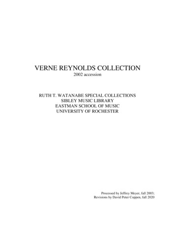
Random (drunkard’s) walk (continued)Random walks behave differently if p 1/2, p 1/2 or p 1/2p 0.50p 0.55100100808080606060404040position (in steps)position (in steps)p 0.45100200 20 40 60position (in steps)I200 20 40 60200 20 40 60 80 80 80 1000 1000 1000100 200 300 400 500 600 700 800 900 1000time100 200 300 400 500 600 700 800 900 1000time100 200 300 400 500 600 700 800 900 1000time With p 1/2 diverges to the right (% almost surely) With p 1/2 diverges to the left (& almost surely) With p 1/2 always come back to visit origin (almost surely)IBecause number of states is infinite we can have all states transientITransient states not revisited after some time (more later)Introduction to Random ProcessesMarkov Chains10
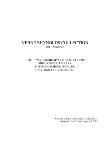
Two dimensional random walk40ITake a step in random direction E, W, S or N35IStates are pairs of coordinates (Xn , Yn )IXn 0, 1, 2, . . . and Yn 0, 1, 2, . . .Latitude (North South)30 E, W, S, N chosen with equal probability2520151050 5Transiton probs. 6 0 only for adjacent pointsEast: P Xn 1 i 1, Yn 1 jWest: P Xn 1 i 1, Yn 1 jNorth: P Xn 1 i, Yn 1 j 1South: P Xn 1 i, Yn 1 j 1Introduction to Random Processes1Xn i, Yn j 4 1Xn i, Yn j 4 1Xn i, Yn j 4 1Xn i, Yn j 4 10 5 Markov Chains0510152025Longitude (East West)303540 40 35 30 25 20 15Longitude (East West) 10 50504030Latitude (North South)I20100 10 20 30 4511
More about random walksISome random facts of life for equiprobable random walksIIn one and two dimensions probability of returning to origin is 1 Will almost surely return homeIIn more than two dimensions, probability of returning to origin is 1 In three dimensions probability of returning to origin is 0.34 Then 0.19, 0.14, 0.10, 0.08, . . .Introduction to Random ProcessesMarkov Chains12
Another representation of a random walkIConsider an i.i.d. sequence of RVs YN Y1 , Y2 , . . . , Yn , . . .IYn takes the value 1, P (Yn 1) p, P (Yn 1) 1 pIDefine X0 0 and the cumulative sumXn nXYkk 1 The process XN is a random walk (same we saw earlier) YN are i.i.d. steps (increments) because Xn Xn 1 YnIQ: Can we formally establish the random walk is a Markov chain?IA: Since Xn Xn 1 Yn , n 1, and Yn independent of Xn 1 P Xn j Xn 1 i, Xn 2 x P Xn 1 Yn j Xn 1 i, Xn 2 x P (Y1 j i) : PijIntroduction to Random ProcessesMarkov Chains13
General result to identify Markov chainsTheoremSuppose YN Y1 , Y2 , . . . , Yn , . . . are i.i.d. and independent of X0 .Consider the random process XN X1 , X2 , . . . , Xn , . . . of the formXn f (Xn 1 , Yn ),n 1Then XN is a Markov chain with transition probabilitiesPij P (f (i, Y1 ) j)IUseful result to identify Markov chains Often simpler than checking the Markov propertyIProof similar to the random walk special case, i.e., f (x, y ) x yIntroduction to Random ProcessesMarkov Chains14
Random walk with boundaries (gambling)IAs a random walk, but stop moving when Xn 0 or Xn JIIModels a gambler that stops playing when ruined, Xn 0Or when reaches target gains Xn J11p0.i 1pi 1i1 pStates are 0, 1, . . . , J, finite number of statesITransition probabilities arePi,i 1 1 p,J1 pIPi,i 1 p,.P00 1,PJJ 1IPij 0 for all other transitionsIStates 0 and J are called absorbing. Once there stay there forever The rest are transient states. Visits stop almost surelyIntroduction to Random ProcessesMarkov Chains15
Chapman-Kolmogorov equationsDefinition and examplesChapman-Kolmogorov equationsGambler’s ruin problemQueues in communication networks: Transition probabilitiesClasses of statesIntroduction to Random ProcessesMarkov Chains16
Multiple-step transition probabilitiesIQ: What can be said about multiple transitions?IEx: Transition probabilities between two time slots Pij2 P Xm 2 j Xm i Caution: Pij2 is just notation, Pij2 6 Pij PijIEx: Probabilities of Xm n given Xm n-step transition probabilities Pijn P Xm n j Xm iIRelation between n-, m-, and (m n)-step transition probabilities Write Pijm n in terms of Pijm and PijnIAll questions answered by Chapman-Kolmogorov’s equationsIntroduction to Random ProcessesMarkov Chains17
2-step transition probabilitiesIStart considering transition probabilities between two time slots Pij2 P Xn 2 j Xn iIUsing the law of total probabilityPij2 X P Xn 2 j Xn 1 k, Xn i P Xn 1 k Xn ik 0IIn the first probability, conditioning on Xn i is unnecessary. ThusPij2 X P Xn 2 j Xn 1 k P Xn 1 k Xn ik 0IWhich by definition of transition probabilities yieldsPij2 XPkj Pikk 0Introduction to Random ProcessesMarkov Chains18
Relating n-, m-, and (m n)-step probabilitiesISame argument works (condition on X0 w.l.o.g., time invariance) Pijm n P Xn m j X0 iIUse law of total probability, drop unnecessary conditioning and usedefinitions of n-step and m-step transition probabilitiesPijm n X P Xm n j Xm k, X0 i P Xm k X0 ik 0Pijm n X P Xm n j Xm k P Xm k X0 ik 0Pijm n XPkjn Pikm for all i, j and n, m 0k 0 These are the Chapman-Kolmogorov equationsIntroduction to Random ProcessesMarkov Chains19
InterpretationIChapman-Kolmogorov equations are intuitive. RecallPijm n XPikm Pkjnk 0IBetween times 0 and m n, time m occurredIAt time m, the Markov chain is in some state Xm k Pikm is the probability of going from X0 i to Xm k Pkjn is the probability of going from Xm k to Xm n j Product Pikm Pkjn is then the probability of going fromX0 i to Xm n j passing through Xm k at time mISince any k might have occurred, just sum over all kIntroduction to Random ProcessesMarkov Chains20
Chapman-Kolmogorov equations in matrix formIDefine the following three matrices: P(m) with elements Pijm P(n) with elements Pijn P(m n) with elements Pijm nIMatrix product P(m) P(n) has (i, j)-th elementIChapman Kolmogorov in matrix formP k 0Pikm PkjnP(m n) P(m) P(n)IMatrix of (m n)-step transitions is product of m-step and n-stepIntroduction to Random ProcessesMarkov Chains21
Computing n-step transition probabilitiesIFor m n 1 (2-step transition probabilities) matrix form isP(2) PP P2IProceed recursively backwards from nP(n) P(n 1) P P(n 2) PP . . . PnIHave proved the followingTheoremThe matrix of n-step transition probabilities P(n) is given by the n-thpower of the transition probability matrix P, i.e.,P(n) PnHenceforth we write PnIntroduction to Random ProcessesMarkov Chains22
Example: Happy-SadIMood transitions in one day0.80.70.2 P 0.8 0.20.3 0.7 HS0.3ITransition probabilities between today and the day after tomorrow?0.700.550.30P2 0.70 0.300.45 0.55 HS0.45Introduction to Random ProcessesMarkov Chains23
Example: Happy-Sad (continued)II. After a week and after a month 0.6031 0.3969P7 0.5953 0.4047P30 0.60000.60000.40000.4000 Matrices P7 and P30 almost identical limn Pn exists Note that this is a regular limitIAfter a month transition from H to H and from S to H w.p. 0.6 State becomes independent of initial condition (H w.p. 0.6)IRationale: 1-step memory Initial condition eventually forgottenIMore about this soonIntroduction to Random ProcessesMarkov Chains24
Unconditional probabilitiesIAll probabilities so far are conditional, i.e., Pijn P Xn j X0 i May want unconditional probabilities pj (n) P (Xn j)IRequires specification of initial conditions pi (0) P (X0 i)IUsing law of total probability and definitions of Pijn and pj (n)pj (n) P (Xn j) X P Xn j X0 i P (X0 i)i 0 XPijn pi (0)i 0IIn matrix form (define vector p(n) [p1 (n), p2 (n), . . .]T )Tp(n) (Pn ) p(0)Introduction to Random ProcessesMarkov Chains25
Example: Happy-Sad ITransition probability matrix P p(0) [1, esProbabilities (0) [0, 1]T0.900.80.30.1051015Time (days)2025300051015Time (days)202530For large n probabilities p(n) are independent of initial state p(0)Introduction to Random ProcessesMarkov Chains26
Gambler’s ruin problemDefinition and examplesChapman-Kolmogorov equationsGambler’s ruin problemQueues in communication networks: Transition probabilitiesClasses of statesIntroduction to Random ProcessesMarkov Chains27
Gambler’s ruin problemIYou place 1 bets(i) With probability p you gain 1, and(ii) With probability q 1 p you loose your 1 betIStart with an initial wealth of iIDefine bias factor α : q/pIIIIIf α 1 more likely to loose than win (biased against gambler)α 1 favors gambler (more likely to win than loose)α 1 game is fairYou keep playing until(a) You go broke (loose all your money)(b) You reach a wealth of N (same as first lecture, HW1 for N )IProb. Si of reaching N before going broke for initial wealth i?IS stands for success, or successful betting run (SBR)Introduction to Random ProcessesMarkov Chains28
Gambler’s Markov chainIModel wealth as Markov chain XN . Transition probabilitiesPi,i 1 p,Pi,i 1 q,P00 PNN 111p0.i 1pi 1iqI.NqRealizations xN . Initial state Initial wealth i Sates 0 and N are absorbing. Eventually end up in one of them Remaining states are transient (visits eventually stop)IBeing absorbing states says something about the limit wealthlim xn 0, orn Introduction to Random Processeslim xn Nn Si : PMarkov Chains lim Xn N X0 i n 29
Recursive relationsITotal probability to relate Si with Si 1 , Si 1 from adjacent states Condition on first bet X1 , Markov chain homogeneousSi Si 1 Pi,i 1 Si 1 Pi,i 1 Si 1 p Si 1 qIRecall p q 1 and reorder termsp(Si 1 Si ) q(Si Si 1 )IRecall definition of bias α q/pSi 1 Si α(Si Si 1 )Introduction to Random ProcessesMarkov Chains30
Recursive relations (continued)IIf current state is 0 then Si S0 0. Can writeS2 S1 α(S1 S0 ) αS1ISubstitute this in the expression for S3 S2S3 S2 α(S2 S1 ) α2 S1IApply recursively backwards from Si Si 1Si Si 1 α(Si 1 Si 2 ) . . . αi 1 S1ISum up all of the former to obtain Si S1 S1 α α2 . . . αi 1IThe latter can be written as a geometric series Si S1 1 α α2 . . . αi 1Introduction to Random ProcessesMarkov Chains31
Probability of successful betting runIGeometric series can be summed in closed form, assuming α 6 1!i 1X1 αikSi α S1 S11 αk 0IWhen in state N, SN 1 and so1 SN I1 α1 αNS1 S1 1 α1 αNSubstitute S1 above into expression for probability of SBR SiSi I1 αi,1 αNα 6 1For α 1 Si iS1 , 1 SN NS1 , Si Introduction to Random ProcessesMarkov ChainsiN32
Analysis for large NIRecall Si I(1 αi )/(1 αN ),i/N,α 6 1,α 1Consider exit bound N arbitrarily large(i) For α 1, Si (αi 1)/αN 0(ii) Likewise for α 1, Si i/N 0IIf win probability p does not exceed loose probability q Will almost surely loose all money(iii) For α 1, Si 1 αiIIf win probability p exceeds loose probability q For sufficiently high initial wealth i, will most likely winIThis explains what we saw on first lecture and HW1Introduction to Random ProcessesMarkov Chains33
Queues in communication systemsDefinition and examplesChapman-Kolmogorov equationsGambler’s ruin problemQueues in communication networks: Transition probabilitiesClasses of statesIntroduction to Random ProcessesMarkov Chains34
Queues in communication systemsIGeneral communication systems goal Move packets from generating sources to intended destinationsIBetween arrival and departure we hold packets in a memory buffer Want to design buffers appropriatelyIntroduction to Random ProcessesMarkov Chains35
Non-concurrent queueITime slotted in intervals of duration t n-th slot between times n t and (n 1) tIAverage arrival rate is λ̄ packets per unit time Probability of packet arrival in t is λ λ̄ tIPackets are transmitted (depart) at a rate of µ̄ packets per unit time Probability of packet departure in t is µ µ̄ tIAssume no simultaneous arrival and departure (no concurrence) Reasonable for small t (µ and λ likely to be small)Introduction to Random ProcessesMarkov Chains36
Queue evolution equationsIQn denotes number of packets in queue (backlog) in n-th time slotIAn nr. of packet arrivals, Dn nr. of departures (during n-th slot)IIf the queue is empty Qn 0 then there are no departures Queue length at time n 1 can be written asQn 1 Qn An ,Iif Qn 0If Qn 0, departures and arrivals may happenQn 1 Qn An Dn ,Iif Qn 0An {0, 1}, Dn {0, 1} and either An 1 or Dn 1 but not both Arrival and departure probabilities areP (An 1) λ,Introduction to Random ProcessesP (Dn 1) µMarkov Chains37
Queue evolution probabilitiesIFuture queue lengths depend on current length onlyIProbability of queue length increasing P Qn 1 i 1 Qn i P (An 1) λ,for all iIQueue length might decrease only if Qn 0. Probability is P Qn 1 i 1 Qn i P (Dn 1) µ,for all i 0IQueue length stays the same if it neither increases nor decreases P Qn 1 i Qn i 1 λ µ,for all i 0 P Qn 1 0 Qn 0 1 λ No departures when Qn 0 explain second equationIntroduction to Random ProcessesMarkov Chains38
Queue as a Markov chainIMC with states 0, 1, 2, . . . Identify states with queue lengthsITransition probabilities for i 6 0 arePi,i 1 µ,IPi,i 1 λ µ,Pi,i 1 λFor i 0: P00 1 λ and P01 λ1 λ µ1 λλλ0.µIntroduction to Random Processes1 λ µ1 λ µi 1λi 1iµµMarkov Chainsλ.µ39
Numerical example: Probability propagationIBuild matrix P truncating at maximum queue length L 100 Arrival rate λ 0.3. Departure rate µ 0.33 Initial distribution p(0) [1, 0, 0, . . .]T (queue empty)010queue length 0queue length 10queue length 20IPropagate probabilities (Pn )T p(0)IProbabilities obtained are P Qn i Q0 0 pi (n) 1Probabilities10 210 3100100200300400Introduction to Random Processes500Time600700800900IA few i’s (0, 10, 20) shownIProbability of empty queue 0.1IOccupancy decreases with i1000Markov Chains40
Classes of statesDefinition and examplesChapman-Kolmogorov equationsGambler’s ruin problemQueues in communication networks: Transition probabilitiesClasses of statesIntroduction to Random ProcessesMarkov Chains41
Transient and recurrent statesIStates of a MC can be recurrent or transientITransient states might be visited early on but visits eventually stopIAlmost surely, Xn 6 i for n sufficiently large (qualifications needed)IVisits to recurrent states keep happening forever. Fix arbitrary mIAlmost surely, Xn i for some n m (qualifications needed)10.2R30.60.2Introduction to Random Processes0.2T10.6T2R10.60.2Markov Chains0.30.7R20.442
DefinitionsILet fi be the probability that starting at i, MC ever reenters state i!! [[fi : PXn i X0 i PXn i Xm in 1In m 1State i is recurrent if fi 1 Process reenters i again and again (a.s.). Infinitely oftenIState i is transient if fi 1 Positive probability 1 fi 0 of never coming back to iIntroduction to Random ProcessesMarkov Chains43
Recurrent states exampleI State R3 is recurrent because it is absorbing P X1 R3 X0 R3 1IState R1 is recurrent because P X1 R1 X0 R1 0.310.2R30.2T10.60.2 P X2 R1 , X1 6 R1 X0 R1 (0.7)(0.6) P X3 R1 , X2 6 R1 , X1 6 R1 X0 R1 (0.7)(0.4)(0.6)0.6R10.6T20.20.30.7R20.4. P Xn R1 , Xn 1 6 R1 , . . . , X1 6 R1 X0 R1 (0.7)(0.4)n 2 (0.6)ISum up: fi XP Xn R1 , Xn 1 6 R1 , . . . , X1 6 R1 X0 R1 n 1 0.3 0.7 X!0.4n 2 0.6 0.3 0.7n 2Introduction to Random ProcessesMarkov Chains11 0.4 0.6 144
Transient state exampleIStates T1 and T2 are transientIProbability of returning to T1 is fT1 (0.6)2 0.36 Might come back to T1 only if it goes to T2 (w.p. 0.6) Will come back only if it moves back from T2 to T1 (w.p. wise, fT2 (0.6)2 0.36Introduction to Random ProcessesMarkov Chains45
Expected number of visits to statesIDefine Ni as the number of visits to state i given that X0 i X Ni : I Xn i X0 in 1IIf Xn i, this is the last visit to i w.p. 1 fiIProb. revisiting state i exactly n times is (n visits no more visits)P (Ni n) fi n (1 fi ) Number of visits Ni 1 is geometric with parameter 1 fiIExpected number of visits isfi1 E [Ni ] 1 fi1 fi For recurrent states Ni a.s. and E [Ni ] (fi 1)E [Ni ] 1 Introduction to Random ProcessesMarkov Chains46
Alternative transience/recurrence characterizationIAnother way of writing E [Ni ]E [Ni ] h i XXE I Xn i X0 i Piinn 1n 1IRecall that: for transient states E [Ni ] fi /(1 fi ) for recurrent states E [Ni ] TheoremP Piin IState i is transient if and only ifIState i is recurrent if and only ifINumber of future visits to transient states is finite If number of states is finite some states have to be recurrentIntroduction to Random ProcessesPn 1 n 1Piin Markov Chains47
AccessibilityIDef: State j is accessible from state i if Pijn 0 for some n 0I It is possible to enter j if MC initialized at X0 i Since Pii0 P X0 i X0 i 1, state i is accessible from itself10.2R30.60.20.2T10.6T2R10.60.20.7R2IAll states accessible from T1 and T2IOnly R1 and R2 accessible from R1 or R2INone other than R3 accessible from itselfIntroduction to Random Processes0.3Markov Chains0.448
CommunicationIDef: States i and j are said to communicate (i j) if j is accessible from i, i.e., Pijn 0 for some n; and i is accessible from j, i.e., Pjim 0 for some mICommunication is an equivalence relationIReflexivity: i iIISymmetry: If i j then j iIIIf i j then Pijn 0 and Pjim 0 from where j iTransitivity: If i j and j k, then i kIIHolds because Pii0 1Just notice that Pikn m Pijn Pjkm 0Partitions set of states into disjoint classes (as all equivalences do) What are these classes?Introduction to Random ProcessesMarkov Chains49
Recurrence and communicationTheoremIf state i is recurrent and i j, then j is recurrentProof.IIf i j then there are l, m such that Pjil 0 and Pijm 0IThen, for any n we havePjjl n m Pjil Piin PijmISum for all n. Note that since i is recurrent Xn 1Pjjl n m XPjil Piin Pijm Pjiln 1P XPiin !n 1PiinPijm n 1 Which implies j is recurrentIntroduction to Random ProcessesMarkov Chains50
Recurrence and transience are class propertiesCorollaryIf state i is transient and i j, then j is transientProof.IIf j were recurrent, then i would be recurrent from previous theoremIRecurrence is shared by elements of a communication class We say that recurrence is a class propertyILikewise, transience is also a class propertyIMC states are separated in classes of transient and recurrent statesIntroduction to Random ProcessesMarkov Chains51
Irreducible Markov chainsIA MC is called irreducible if it has only one classIIIIWhen it has multiple classes (not irreducible)IIIIAll states communicate with each otherIf MC also has finite number of states the single class is recurrentIf MC infinite, class might be transientClasses of transient states T1 , T2 , . . .Classes of recurrent states R1 , R2 , . . .If MC initialized in a recurrent class Rk , stays within the classIf MC starts in transient class Tk , then it might(a) Stay on Tk (only if Tk )(b) End up in another transient class Tr (only if Tr )(c) End up in a recurrent class RlIFor large time index n, MC restricted to one class Can be separated into irreducible componentsIntroduction to Random ProcessesMarkov Chains52
Communication classes hree classes T : {T1 , T2 }, class with transient states R1 : {R1 , R2 }, class with recurrent states R2 : {R3 }, class with recurrent stateIFor large n suffices to study the irreducible components R1 and R2Introduction to Random ProcessesMarkov Chains53
Example: Random walkIStep right with probability p, left with probability q 1 pp.pi 11 pp.i 1i1 pp1 p1 pIAll states communicate States either all transient or all recurrentITo see which, consider initially X0 0 and note for any n 1 2n n n(2n)! n n2nP00 p q p qnn!n! Back to 0 in 2n steps n steps right and n steps leftIntroduction to Random ProcessesMarkov Chains54
Example: Random walk (continued)I Stirling’s formula n! nn ne n 2π2nof returning home as Approximate probability P002nP00 I(2n)! n n(4pq)np q n!n!nπSymmetric random walk (p q 1/2) X2nP00 n 1 Xn 11 nπ State 0 (hence all states) are recurrentIBiased random walk (p 1/2 or p 1/2), then pq 1/4 and Xn 12nP00 X(4pq)n nπn 1 State 0 (hence all states) are transientIntroduction to Random ProcessesMarkov Chains55
Example: Right-biased random walkIAlternative proof of transience of right-biased random walk (p 1/2)p.i 11 pIpp.i 1i1 pp1 pWrite current position of random walker as Xn 1 pPnk 1Yk Yk are the i.i.d. steps: E [Yk ] 2p 1, var [Yk ] 4p(1 p)IFrom Central Limit Theorem (Φ(x) is cdf of standard Normal)!Pnk 1 Yk n(2p 1)pP a Φ(a)n4p(1 p)Introduction to Random ProcessesMarkov Chains56
Example: Right-biased random walk (continued) IChoose a n(1 2p) 0, use Chernoff bound Φ(a) exp( a2 /2)4p(1 p)P (Xn 0) PnX! n(1 2p)2n(1 2p)p e 8p(1 p) 04p(1 p)!Yk 0 Φk 1InSince P00 P (Xn 0), sum over n Xn 1InP00 XP (Xn 0) n 1 Xn(1 2p)2e 8p(1 p) n 1This establishes state 0 is transient Since all states communicate, all states are transientIntroduction to Random ProcessesMarkov Chains57
Take-home messagesIStates of a MC can be transient or recurrentIA MC can be partitioned into classes of communicating states Class members are either all transient or all recurrent Recurrence and transience are class properties A finite MC has at least one recurrent classIA MC with only one class is irreducible If reducible it can be separated into irreducible componentsIntroduction to Random ProcessesMarkov Chains58
GlossaryIMarkov chainICommunication systemIState spaceINon-concurrent queueIMarkov propertyIQueue evolution modelITransition probability matrixIRecurrent and transient statesIState transition diagramIAccessibilityIState augmentationICommunicationIRandom walkIEquivalence relationIn-step transition probabilitiesICommunication classesIChapman-Kolmogorov eqs.IClass propertyIInitial distributionIIrreducible Markov chainIGambler’s ruin problemIIrreducible componentsIntroduction to Random ProcessesMarkov Chains59
Random (drunkard’s) walk I Step to the right w.p. p, to the left w.p. 1 p)Not that drunk to stay on the same place::: 1i 1 ::: p 1 p 1 p p p 1 p 1 p p I States are 0; 1; 2;:::(state space is Z),in nite number of states I Transition probabilities are P i;i 1 p; P i;i 1 1 p I P ij