Transcription
2 Working with Microsoft Excel 2016LESSON SKILL MATRIXSkillsExam ObjectiveObjective NumberCreating WorkbooksCreate a workbook.1.1.1Saving WorkbooksSave workbooks in alternative file formats.Inspect a workbook for compatibility issues.1.5.21.5.8Entering and Editing Basic Data in a WorksheetReplace data.Adjust row height and column width.Fill cells by using Auto Fill.Insert and delete cells.2.1.11.3.72.1.42.1.5Using Data Types to Populate a WorksheetApply number formats.2.2.5Cutting, Copying, and Pasting DataCut, copy, or paste data.2.1.2Editing a Workbook’s PropertiesModify document properties.1.4.6SOFTWARE ORIENTATIONExcel’s Home TabThe ribbon in Microsoft Office Excel 2016 is made up of a series of tabs, each related to specifickinds of tasks that you perform in Excel. The Home tab, shown in Figure 2-1, contains the commands that people use the most when creating Excel documents. Having commands visible onthe work surface enables you to see at a glance most tasks you want to perform. Each tab containsgroups of commands related to specific tasks or functions.CutPasteCopyCommand Dialog Box launchersCommand groupsCommand button arrowsFormula b arFigure 2-1Ribbon, formula bar, andcommand optionsSome commands have an arrow associated with them. In Figure 2-1, you see the button arrowsassociated with AutoSum and Find & Select. This indicates that in addition to the default task,other options are available for the task. Similarly, some of the groups have Dialog Box Launchersassociated with them. Clicking these displays additional commands not shown on the ribbon. InFigure 2-1, the Clipboard, Font, Alignment, and Number groups have associated dialog boxes ortask panes, whereas Styles, Cells, and Editing do not.1212
Working with Microsoft Excel 201613CREATING WORKBOOKSThere are three ways to create a new Microsoft Excel workbook. You can open a new, blank workbook when you launch Excel or by using the File tab to access Backstage view. You can open anexisting Excel workbook, enter new or additional data, and save the file with a new name, thuscreating a new workbook. You can also use a template to create a new workbook. A template is amodel that has already been set up to display certain kinds of data, such as sales reports, invoices,and so on.Creating a Workbook from ScratchTo create a new workbook, launch Excel and select a blank workbook or another type of template.If you are working in Excel and want to begin a new workbook, click the File tab, click New, andthen click Blank workbook. Worksheets often include text that describes the content of the worksheet. In this exercise, you create two Excel workbooks: one with a company address and one witha quick phone message.STEP BY STEPCreate a Workbook from ScratchGET READY. LAUNCH Excel. Excel gives you options for starting a blank workbook, takinga tour, or using templates (see Figure 2-2).Figure 2-2Available options after Excelis launched1. Click Blank workbook. If you have just launched Excel, Book1 – Excel appears in thetitle bar at the top of the window. A blank workbook opens with A1 as the active cell.2. In cell A1, type Fabrikam Inc. This entry is the primary title for the worksheet. Note thatas you type, the text appears in the cell and in the formula bar (see Figure 2-3). See thedefinition of formula bar in the “Editing a Cell’s Contents” section, later in this lesson.
14Lesson 2Figure 2-3Typed text appears in boththe active cell and theformula bar.Formula barActive cell3. Press Enter. The text is entered into cell A1, but appears as if it flows into cell B1.4. In cell A2, type 123 Fourth Street and then press Enter.5. In cell A3, type Columbus, OH 43204 and then press Enter.6. Sometimes you need a quick work area to complete another task while you are in themiddle of a workbook. You can open another workbook as a scratch area. Click the Filetab, and in the left pane, click New. The different templates available appear (refer toFigure 2-2).7. In the Backstage view, click Blank workbook. A second Excel workbook opens andBook2 appears in the title bar.8. In cell A1, type Phone Calls and then press Enter.9. In cell A2, type David Ortiz UA flight 525 arriving 4:30 pm and then press Enter.10. Click the File tab to open Backstage view. In the left pane, click Close to close the PhoneCalls workbook. In the message box, click Don’t Save.PAUSE. LEAVE the Fabrikam workbook open for the next exercise.SAVING WORKBOOKSWhen you save a file, you can save it to a folder on your computer’s hard drive, a network drive,disc, CD, USB drive, OneDrive, or other storage location. You must first identify where the document is to be saved. The remainder of the Save process is the same, regardless of the location orstorage device.Naming and Saving a WorkbookWhen you save a file for the first time, you are asked two important questions: Where do youwant to save the file? What name will you give to the file? In this lesson, you practice answeringthese questions for two different files. By default in all Office applications, documents are saved tothe Documents folder or to your OneDrive, depending on settings specified during the programinstallation.
Working with Microsoft Excel 2016STEP BY STEP15Name and Save a WorkbookGET READY. USE the workbook from the previous exercise.1. Click the File tab to open Backstage view. In the left pane, click Save As to display thesave options.2. Double-click This PC to open the Save As dialog box (see Figure 2-4).Figure 2-4Save As dialog box3. In the navigation pane on the left, in the Save As dialog box, click Desktop. TheDesktop becomes the new destination of your saved file.4. In the Save As dialog box, click New folder. A folder icon appears with the words Newfolder selected.5. Type Excel Lesson 2 and then press Enter.6. Click the Open button.7. In the File name box, type 02 Fabrikam Address Solution.8. Click the Save button.PAUSE. LEAVE the workbook open to use in the next exercise.Take NoteSave your workbook often and especially before opening another workbook, printing, or after youenter information.Saving to Your OneDriveOneDrive is a cloud-based application that allows you to store and sync your files so you can retrieve them anywhere and share them with other people if desired. OneDrive is also a great placeto store backup files of important documents. OneDrive comes with recent versions of Windowsand Microsoft Office. A free desktop app is also available for mobile devices. This exercise assumesyou already have access to OneDrive.
16Lesson 2STEP BY STEPSave to Your OneDriveGET READY. USE the workbook from the previous exercise.1. Click the File tab and then click Save As.2. In the Backstage view, under Save As, click your OneDrive account, and then click afolder location in the right pane. You may need to sign in to OneDrive if you haven’talready (see Figure 2-5).Select your OneDriveSelect a folder locationSign in to OneDrive, if promptedFigure 2-5OneDrive informationin Backstage view3. Click the New folder button in the Save As dialog box.4. In the New folder text box, type Excel Lesson 2 to save a folder for this lesson on yourOneDrive and then press Enter.5. Double-click the Excel Lesson 2 icon to move to that folder.6. Keep the file with the same name (or type 02 Fabrikam Address Solution in the Filename box), and then click the Save button.PAUSE. LEAVE the workbook open to use in the next exercise.Saving a Workbook Under a Different NameYou can rename an existing workbook to create a new workbook. For example, when you havemultiple offices, you can save a file with a new name and use it to enter data for another office. Youcan also use an existing workbook as a template to create new workbooks. In this exercise, youlearn how to use the Save As dialog box to implement either of these options.STEP BY STEPSave a Workbook Under a Different NameGET READY. USE the workbook from the previous exercise.1. In cell A2, type 87 East Broad Street and then press Enter.2. In cell A3, type Columbus, OH 43215 and then press Enter.3. Click the File tab, and in the left pane, click Save As. The Backstage view shows that theCurrent Folder in the right pane is Excel Lesson 2 on your OneDrive, because it was thefolder that was last used to save a workbook.
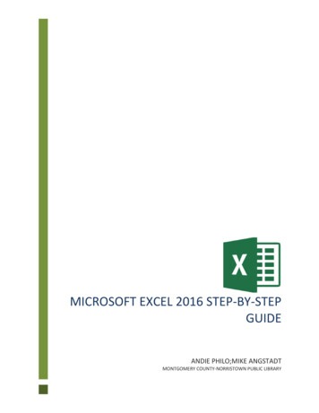
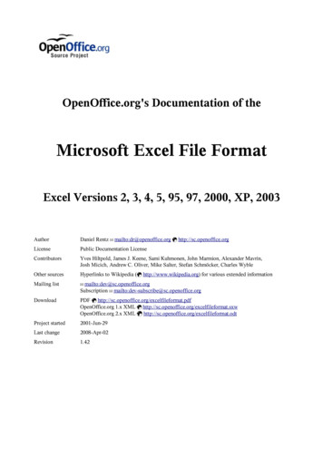
Working with Microsoft Excel 2016174. Click This PC to return to the drive you used before.5. In the right pane, click Excel Lesson 2.6. Click in the File name box, click after Fabrikam, and then type Broad so the name reads02 Fabrikam Broad Address Solution.7. Click Save. You created a new workbook by saving an existing workbook with a newname.8. Click the File tab, click Save As in the left pane, and then click Browse.9. In the File name box, type 02 Fabrikam Broad Address Template Solution.10. In the Save as type box, click the drop-down arrow and then choose Excel Template.Click the Save button.Take NoteTemplates are automatically saved in another location so they can be opened with the File, Newoption.PAUSE. CLOSE Excel.Creating a template to use for each new workbook based on the example file eliminates the possibility that you might lose data because you might overwrite a file after you enter new data. To usethe template, you choose File New Personal and select the template you saved. When you exit,you are prompted to save the file with a new name.Saving a Workbook in a Previous Excel FormatFiles created in earlier Excel versions can be opened and revised in Excel 2016. However, if some ofyour users do not have the latest version or use other applications, they might not be able to openyour file. You can save a copy of an Excel 2016 workbook (with the .xlsx file extension) to the olderExcel 97-2003 Workbook format (with the .xls file extension). The program symbol displayed withthe filenames is different, but it is a good idea to give the earlier edition file a different name. It isalso a good idea to check which features might be lost with Excel’s compatibility checker.STEP BY STEPSave a Workbook in a Previous Excel FormatGET READY. LAUNCH Excel.1. At the bottom of the left pane, click Open Other Workbooks.2. In the list of recent files in the right pane, click 02 Fabrikam Broad Address Solution.3. First check for compatibility issues. Click the File tab, click Info, click Check for Issues,and then click Check Compatibility. The Microsoft Excel - Compatibility Checker dialogbox in Figure 2-6 opens.Figure 2-6The Compatibility Checkershowing no compatibilityissues
18Lesson 24. Read the information in the Compatibility Checker dialog box and then click OK.5. Click the File tab, click Export, and then click Change File Type. The Backstage viewshows the different file types (see Figure 2-7).Figure 2-7Change File Type options inBackstage view6. Click Excel 97-2003 Workbook and then click Save As.7. In the File name box, click before Solution, type 97-03, and then click Save.8. Click the File tab, and then click Close to close the 02 Fabrikam Broad Address 97-03Solution workbook.9. Click the File tab and then click Open. The right pane in Backstage view shows the lastset of documents that have been saved.10. Click 02 Fabrikam Broad Address Solution.PAUSE. LEAVE the workbook open to use in the next exercise.Saving in Different File FormatsYou can save an Excel 2016 file in a format other than .xlsx or .xls. The file formats that are listedas options in the Save As dialog box or on the Export tab depend on what type of file format theapplication supports. When you save a file in another file format, some of the formatting, data,and features might be lost.STEP BY STEPSave in Different File FormatsGET READY. USE the 02 Fabrikam Broad Address Solution workbook from the previousexercise or type your name and address in a new workbook.1. Click the File tab, and then click the Export button.2. Click the Change File Type button. Excel explains the different file types (refer toFigure 2-7).3. Click the Create PDF/XPS Document option. Figure 2-8 shows the reasons for usingthis format.
Working with Microsoft Excel 201619Figure 2-8Backstage view withinformation about thePDF/XPS format4. In the right pane, click the Create PDF/XPS button.5. In the left navigation pane, click Desktop.6. Double-click Excel Lesson 2 to move to that folder.7. In the Publish as PDF or XPS dialog box, ensure that the Save as type list shows PDF.8. Click Publish.9. The Reader application (or a Web browser) opens with the PDF file displayed.10. Press Alt F4 to close the browser or Reader application.11. If necessary, press Alt Tab to return to the Excel file.PAUSE. CLOSE the workbook and LEAVE Excel open to use in the next exercise.Take NoteAdobe PDF (Portable Documents Format) ensures that your printed or viewed file retains theformatting that you intended, but the file cannot be easily changed. You can also save your workbooks in a Web page format for use on websites with the Single File Web Page or Web Page optionsin the Save As dialog box. To import data into another format, you can also try Text (Tab delimited) or CSV (Comma delimited) formats. All of these options are available from the Save as typedrop-down list or the Export tab.ENTERING AND EDITING BASIC DATA IN A WORKSHEETYou can type data directly into a worksheet cell. You can also copy and paste information fromanother worksheet or from other programs. Copy takes the information from one location andduplicates it. You use Paste to put this information into another location. To enter data in a cellin a worksheet, you must make the desired cell active and then type the data. To move to the nextcolumn after text is entered, press Tab. Continue to press Tab to go to the next column.Entering Basic Data in a WorksheetWhen you finish typing the entries in a row, press Enter to move to the beginning of the nextrow. You can also use the arrow keys to move to an adjacent cell or click on any cell to make thatcell active. Press Enter to accept the entry and move down one row. In the following exercise, youcreate a list of people working in the office.
20Lesson 2STEP BY STEPEnter Basic Data in a WorksheetGET READY. If necessary LAUNCH Excel and OPEN a new workbook.1. Click cell A1, type Fabrikam Inc., and then press Enter. Notice that the active cell movesto the next row, to cell A2.2. In cell A2, type Employee List and then press Enter.3. Click cell A4, type Name, and then press Tab. Notice that the active cell moves to thenext column, to cell B4.TroubleshootingIf you type the wrong data, you can click the cell and retype the entry. In the following sections, you see how to edit text.4. Type Extension and then press Enter. Notice that the active cell moves to the first cellin the next row.5. Type Richard Carey and then press Tab.6. Type 101 and then press Enter. Richard Carey’s name looks cut off.7. Click cell A5 and notice that the complete entry for Richard Carey appears in theformula bar.8. Click cell A6, type David Ortiz, and then press Enter.9. Type Kim Akers and then press Enter.10. Type Nicole Caron and then press Enter.11. SAVE the workbook in the Excel Lesson 2 folder on your computer as 02 FabrikamEmployees Solution. Your file should look like Figure 2-9.Figure 2-9The completed 02 FabrikamEmployees workbookPAUSE. LEAVE the workbook open for the next lesson.Take NoteText is stored in only one cell, even when it appears to extend into adjacent cells. If an entry islonger than the cell width and the next cell contains data, the entry appears in truncated form. Toedit the data, you need to go to the cell where the text starts and not to the adjacent cells.Changing the Column WidthIn Excel, column width is established based on the existing data. When you add an entry in acolumn that extends beyond the column’s width, it is necessary to adjust the column width toaccommodate the entry.STEP BY STEPChange the Column WidthGET READY. Use the 02 Fabrikam Employees Solution file from the previous exercise.1. Move the mouse pointer between columns A and B, to the column markers at the top ofthe worksheet (see Figure 2-10). The mouse pointer changes to a double-headed arrow.
Working with Microsoft Excel 201621Figure 2-10Resizing a columnDouble-headed arrow2. Double-click the column marker between A and B. The width of the column changesto the widest entry in column A. In this case, the widest entries are Employee List andRichard Carey’s name.Take NoteTo change the column width manually, point to the column marker between columns A and Band drag the pointer left or right instead of double-clicking.3. Drag the double-headed arrow mouse pointer between columns B and C until theScreenTip shows Width: 20 (145 pixels) or something close to this amount (seeFigure 2-11), and then release the mouse button.Figure 2-11When you drag the double-headed arrow pointer, theScreenTip shows the columnwidth.4. SAVE the 02 Fabrikam Employees Solution file. This overwrites your previous versionwithout the column width change.PAUSE. CLOSE the workbook and LEAVE Excel open for the next exercise.Take NoteWhen you type text that is longer than the cell’s width, the text appears as if it extends into thenext cell. However, when you type in the next cell, the overflow text does not display. The text isstill there. It is often easier to proof your work if you have the column widths match the longesttext entries. You can double-click on the column markers to automatically adjust to the widestentry or drag the column marker to adjust the column width to your desired width.Editing a Cell’s ContentsOne advantage of electronic records versus manual records is that changes can be made quicklyand easily. To edit information in a worksheet, you can make changes directly in the cell or editthe contents of a cell in the formula bar, located between the ribbon and the worksheet. Whenyou enter data in a cell, the text or numbers appear in the cell and in the formula bar. You canalso enter data directly in the formula bar. Before changes can be made, however, you must select
22Lesson 2the information that is to be changed. Selecting text means that you highlight the text that isto be changed. You can select a single cell or a portion of the cell’s text in the formula bar beforeyou make changes. You can also double-click in a cell to position the insertion point for editing.STEP BY STEPEdit a Cell’s ContentsGET READY. OPEN a blank workbook.1. Click cell A1, type Fabrikam, and then press Enter. The insertion point moves to cell A2and nothing appears in the formula bar.2. Click cell A1. Notice that the formula bar displays Fabrikam (see Figure 2-12).Figure 2-12Active cell and formula bar displaying thesame informationFormula barActive cell3. Click after Fabrikam in the formula bar, type a space, type Incorporated, and then pressTab. The insertion point moves to cell B1 and nothing appears in the formula bar (seeFigure 2-13).Figure 2-13Although it looks like text isin B1, it is actually extendedtext from A1.Nothingshows in theformula bar.4. Click cell A1 and in the formula bar, double-click on Incorporated to select it. Type Inc.and then press Enter.5. Type Sales and then press Enter.6. Click cell A2 and then click after Sales in the formula bar.7. Press Home. The insertion point moves to the beginning of the formula bar.
Working with Microsoft Excel 2016Take Note23While you are editing in the formula bar, you can press Home to move to the beginning, End tomove to the end, or the left or right arrow keys to move one character at a time. Press Delete todelete characters after the insertion point. Press Backspace to delete characters before the insertionpoint.8. Type Monthly and then press the spacebar. Press Enter.9. In cell A3, type January and then press Enter.10. Click cell A3, type February, and then press Enter. Cell A3’s original text is gone andFebruary replaces January.11. Click cell A3 and then press Delete. The entry in A3 is removed.12. Above row 1 and to the left of column A, click the Select All button. All cells on theworksheet are selected.13. Press Delete. All entries are removed.PAUSE. CLOSE the workbook without saving and LEAVE Excel open for the next exercise.Take NoteIf you edit a cell’s contents and change your mind before you press Enter, press Esc and the original text will be restored. If you change the contents of a cell, press Enter, and then do not want thechange, click the Undo button on the Quick Access Toolbar or press Ctrl Z. The previous entrywill be restored.You can edit a cell by double-clicking the cell and then typing the replacement text in the cell. Or,you can click the cell and then click in the formula bar.When you are in Edit mode: The insertion point appears as a vertical bar and most commands are inactive. You can move the insertion point by using the left and right arrow keys. The Edit indicator appears at the left end of the Status bar.Use the Home key on your keyboard to move the insertion point to the beginning of the cell, anduse the End key to move the insertion point to the end of the cell. You can add new characters atthe location of the insertion point.To select multiple characters while in Edit mode, press Shift while you press the arrow keys. Youalso can use the mouse to select characters while you are editing a cell. Just click and drag themouse pointer over the characters that you want to select.As in the preceding exercises, there are several ways to modify the values or text you enter into acell: Erase the cell’s contents. Replace the cell’s contents with something else. Edit the cell’s contents.Deleting and Clearing a Cell’s ContentsTo erase the entire contents of a cell, click the cell and then press Delete. This deletes what is in thecell rather than the cell itself. To erase the contents of more than one cell, select all the cells thatyou want to erase and on your keyboard, press Delete. Pressing Delete removes the cell’s contents,but does not remove any formatting (such as bold, italic, or a different number format) that youmight have applied to the cell.
24Lesson 2STEP BY STEPDelete and Clear a Cell’s ContentsGET READY. OPEN a blank workbook.1. In cell A1, type 1 and then press Enter.2. Type 2 and then press Enter.3. Type 3 and then press Enter.4. Type 4 and then press Enter.5. Highlight cells A1 through A4 (containing the numbers 1 through 4).6. Press Delete. All the cells are erased.7. On the Quick Access Toolbar, click the Undo button to restore the cell entries.8. Click cell B5, type 275,000, and then press Enter. The value and format are placed intothe cell.9. Click cell B5 and then press Delete.10. Type 225000 without the dollar sign and comma and then press Enter. Notice that 225,000 is formatted. Although the original entry is gone, the cell retains the previousformat when you press Delete.11. Click cell B5 and on the Home tab, in the Editing group, click Clear.12. Click Clear Formats. Cell B5 displays 225000 without the dollar sign and comma.Take NoteClear displays a number of options. To remove both the entry and the format, choose Clear All.PAUSE. CLOSE the workbook without saving and LEAVE Excel open for the next exercise.USING DATA TYPES TO POPULATE A WORKSHEETYou can enter three types of data into Excel: text, numbers, and formulas. You have already entered basic text and numeric data in this lesson. In the following exercises, you enter dates, useAuto Fill to complete data in a series, and use the Flash Fill feature to speed data entry down acolumn. You enter formulas in Lesson 4, “Using Basic Formulas.” Text entries contain alphabeticcharacters and any other characters that do not have a purely numeric value. The strength of Excel is its capability to calculate and analyze numbers based on the numeric values you enter. Ofcourse, if you enter the wrong numbers, you get the wrong calculations. For that reason, accuratedata entry is crucial.Entering DatesDates are often used in worksheets to track data over a specified period of time. Like text, datescan be used as row and column headings. However, dates are considered serial numbers, whichmeans that they are sequential and can be added, subtracted, and used in calculations. Dates canalso be used in formulas and in developing graphs and charts. The way a date is initially displayedin a worksheet cell depends on the format in which you type the characters. In Excel 2016, the default date format uses four digits for the year. Also by default, dates are right-justified in the cells.STEP BY STEPEnter DatesGET READY. OPEN 02 Fabrikam Sales from the data files for this lesson.1. Click cell B5, type 1/4/2017, and then press Enter.2. Click cell B6, type 1/25/17, and then press Enter. The date is entered in B6 as 1/25/2017and B7 becomes the active cell.3. Type 1/23 and then press Enter. 23-Jan is entered in the cell. Click cell B7, and noticethat 1/23/20XX (with XX representing the current year) appears in the formula bar.
Working with Microsoft Excel 2016254. If the year displayed in the formula bar is not 2017, click cell B7 and then press F2.Change the year to 2017 and then press Enter.5. In cell B8, type 1/28/17 and then press Enter.6. In cell B9, type January 21, 2017 and then press Enter. 21-Jan-17 appears in the cell. Ifyou enter a date in a different format than specified or had already entered somethingin the cell and deleted it, your worksheet might not reflect the results described. Thedate formats in column B are not consistent (see Figure 2-14). You apply a consistentdate format in the next section.Figure 2-14If you don’t type dates thesame way, the formats areinconsistent in a workbook.7. In cell B9, type 1/1/17 and then press Enter. Notice that the value changes but theformatting remains the same.8. Click the Undo button to return to the workbook shown in Figure 2-14.PAUSE. LEAVE the workbook open to use in the next exercise.Excel interprets two-digit years from 00 to 29 as the years 2000 to 2029; two-digit years from 30to 99 are interpreted as 1930 to 1999. If you enter 1/28/28, the date will be displayed as 1/28/2028in the cell. If you enter 1/28/37, the cell will display 1/28/1937.If you type January 28, 2020, the date will display as 28-Jan-20. If you type 1/28 without a year,Excel interprets the date to be the current year. 28-Jan will display in the cell, and the formula barwill display 1/28/ followed by the current four-digit year. In the next section, you learn to apply aconsistent format to a series of dates.Take NoteWhen you enter a date into a cell in a particular format, the cell is automatically formatted even ifyou delete the entry. Subsequent numbers entered in that cell will be converted to the date formatof the original entry.Regardless of the date format displayed in the cell, the formula bar displays the date in month/day/four-digit-year format because that is the format required for calculations and analyses.Filling a Series with Auto FillExcel provides Auto Fill options that automatically fill cells with data and/or formatting. Topopulate a new cell with data that exists in an adjacent cell, use the Auto Fill feature either throughthe command or the fill handle. The fill handle is a small green square in the lower-right cornerof a selected cell or range of cells. A range is a group of adjacent cells that you select to performoperations on all of the selected cells. When you refer to a range of cells, the first cell and last cellare separated by a colon (for example, C4:H4).To use the fill handle, point to the lower-right corner of the cell or range until the mouse pointerturns into a . Click and drag the fill handle from cells that contain data to the cells you want tofill with that data, or have Excel automatically continue a series of numbers, numbers and textcombinations, dates, or time periods, based on an established pattern. To choose an interval for
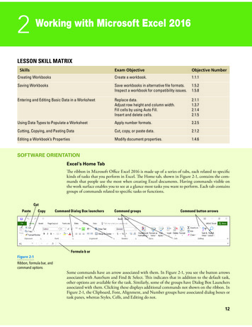
26Lesson 2your series, type the first two entries, select them, and then use the fill handle to expand the seriesusing the pattern of the two selected cells. In this exercise, you use the Auto Fill command and fillhandle to populate cells with data.STEP BY STEPFill a Series with Auto FillGET READY. USE the workbook from the previous exercise or type the text in Figure 2-14.1. Select the range C4:H4. January is in the first cell.2. On the Home tab, in the Editing group, click the Fill button. The Fill menu appears (seeFigure 2-15).Figure 2-15Fill drop-down menuFill buttonFill options3. From the menu, click Right. The contents of C4 (January) are filled into all the cells.4. Click the Undo button.5. Select the range C9:C13 and then click the Fill button. Choose Down. The content of C9is copied into the four additional cells.6. Click the Undo button.7. Click cell C4, point to the fill handle in the lower-right corner of the cell (see Figure 2-16),and drag it to E4 and release. The Auto Fill Options button appears next to the range,and January through March are displayed.Figure 2-16Mouse pointer changes to ablack in the lower-right cornerof a selected cell or rangeFill handle8. Click cell C5, point to the fill handle, and then drag it to C9 and release. All the numbersturn to 275,000 in column C. The Auto Fill Options button appears near the lower-rightcorner of the selected range (see Figure 2-17).9. Click the Auto Fill Options button, and choose Fill Formatting Only from the list thatappears. All the numbers return to their previous values and are formatted with dollarsigns and commas.10. Repeat Steps 8 and 9 for the range B5:B9.
Working with Microsoft Excel 201627Figure 2-17You can fill numbers, formats,or other options.Auto Fill Optionsbutton11. Click cell A9, and then drag the fill handle down to A15. Ryan Calafato’s name isrepeated.12. Click the Undo button to return the spreadsheet.13. SAVE the workbook as 02 Fabrikam Sales Solution.PAUSE. CLOSE the workbook and LEAVE Excel open for the next exercise.After you fill cells using the fill handle, the Auto Fill
Working with Microsoft Excel 2016 13 CREATING WORKBOOKS ere are three ways to create a new Microsoft Excel workbook. You can open a new, blank work-book when you launch Excel or by using the File tab to access Backstage view. You can open an existing Excel workbook, enter new o