Transcription
Université Libre de BruxellesThe TESLA coil2ndChristopher Gerekos,year Physics undergraduate student.“Let the future tell the truth and evaluate each one according to his work and accomplishments.The present is theirs; the future, for which I really worked, is mine.”-Nikola Tesla2011-2012
Special thanksThis Tesla coil never would have existed without my friend Mael Flament, former student at the UniversitéLibre de Bruxelles, now studying at the Hawaii University (Manoa). He initiated the idea of this projectand taught me the basics of electrical engineering and crafting.I also thank Kevin Wilson, creator of the TeslaMap program and webmaster of Tesla Coil Design,Construction and Operation Guide i , which were my main guides during the early stages of the conceptionand construction of the coil. He also proofread this English version of the present document.Thanks to Thomas Vandermergel for his participation in the Printemps des Sciences fair and to JeanLouis Colot for his guidance and his awesome photographs of Zeus.I also express my full gratitude to my family for their support.i Referencedin the Bibliography.
Contents1 Introduction12 The Zeus Project33 Theory of operation3.1 Reminder of the basics . . . . . . . . . . . . . . . . . . . . . . .3.1.1 Resistor . . . . . . . . . . . . . . . . . . . . . . . . . . .3.1.2 Capacitor . . . . . . . . . . . . . . . . . . . . . . . . . .3.1.3 Inductor . . . . . . . . . . . . . . . . . . . . . . . . . . .3.1.4 Impedance . . . . . . . . . . . . . . . . . . . . . . . . .3.2 LC circuit . . . . . . . . . . . . . . . . . . . . . . . . . . . . . .3.2.1 Impedance . . . . . . . . . . . . . . . . . . . . . . . . .3.2.2 Resonant frequency . . . . . . . . . . . . . . . . . . . .3.2.3 RLC circuit . . . . . . . . . . . . . . . . . . . . . . . . .3.3 Tesla coil operation . . . . . . . . . . . . . . . . . . . . . . . . .3.3.1 Description of a cycle . . . . . . . . . . . . . . . . . . .3.3.2 Voltage gain . . . . . . . . . . . . . . . . . . . . . . . . .3.3.3 Comparison with the induction transformer . . . . . . .3.3.4 Distribution of capacitance within the secondary circuit3.3.5 Influence of the coupling . . . . . . . . . . . . . . . . . .3.3.6 A few words on the three-coil transmitter . . . . . . . .3.4 The quarter-wave antenna . . . . . . . . . . . . . . . . . . . . .3.4.1 Comparison with the Tesla coil . . . . . . . . . . . . . .55566781213131515192021222324244 Conception and construction4.1 HV transformer . . . . . . .4.1.1 Arc length . . . . . .4.2 Primary circuit . . . . . . .4.2.1 Capacitor . . . . . .4.2.2 Charge at resonance4.2.3 Inductance . . . . .4.3 Spark gap . . . . . . . . . .4.4 Secondary circuit . . . . . .4.4.1 Coil . . . . . . . . .4.4.2 Top load . . . . . . .4.5 Resonance tuning . . . . . .4.6 RF ground . . . . . . . . .4.7 Other components . . . . .2626282929363842454548515253.
viCONTENTS4.84.7.1 NST protection4.7.2 PFC capacitor4.7.3 AC line filter .Last step . . . . . . .filter. . . . . . .535456565 Nikola Tesla, a mind ahead of its time.57Appendices59A Specifications of the Zeus Tesla coil60B Behavior of the signal in the secondary coil63C Analysis of the RLC circuit65D Analysis of two inductively coupled oscillating circuits.67D.1 Two coupled LC circuits . . . . . . . . . . . . . . . . . . . . . . . . . . . . . . . . . . . . . . 67D.2 Two coupled RLC circuits . . . . . . . . . . . . . . . . . . . . . . . . . . . . . . . . . . . . . 70References75Bibliography76
Chapter 1IntroductionThe device we now call a "Tesla coil" is probably the most famous invention of Nikola Tesla. On the patenthe submitted in 1914 to the US Patent & Trademark Office, it was called "Appartus for transmittingelectrical energy" iNikola Tesla was born the 10th of July 1856 in a Serbian village of the Austrian Empire (in today’sCroatia) and died the 7th of January 1943 in the United States [1].It is not an exaggeration to say he was a visionary who changed the world. With his works onalternative current, including many patents on generators, transformers and turbines, he allowed thewidespread proliferation of electricity as a source of power as we know it today.He was also a pioneer in the domain of telecommunications ; the Tesla coil can be viewed as one ofthe very first attempts of a radio antenna. It consisted of circuits that are fundamentally the same as ourmodern wireless devices.Figure 1.2: His first laboratory in Colorado Springs.[Photographs : Wikimedia Commons]Figure 1.1: Nikola Tesla in 1890.i Thefront picture is a drawing associated with this patent. See Bibliography.1
2CHAPTER 1. INTRODUCTIONDocument structureThis document is about the theory of operation of Tesla coils as well as the specific behavior of its individualcomponents. It also relates the steps of the construction of my own first coil, Zeus.We will only discuss the conventional Tesla coil, consisting of a spark gap and two tank circuits andcalled Spark Gap Tesla Coil (SGTC). In fact, Nikola Tesla also conceived a more advanced type of coil,the magnifying transmitter, which is made of three coils instead of two and which operates in a slightlymore complicated manor. In addition, there is also a class of semiconductors-controlled Tesla coils calledSolid State Tesla Coils (SSTC), which are structurally different but share the same theoretical basis of theconventional Tesla coil.To fully appreciate this document, it is recommended that you master the fundamental concepts ofelectromagnetism and alternating currentii , as well as the basics of differential equations.ii All About Circuits (http://www.allaboutcircuits.com) is an excellent on-line resource. Volumes I and II largely spanthe "engineering" part of the aforementioned perquisites.
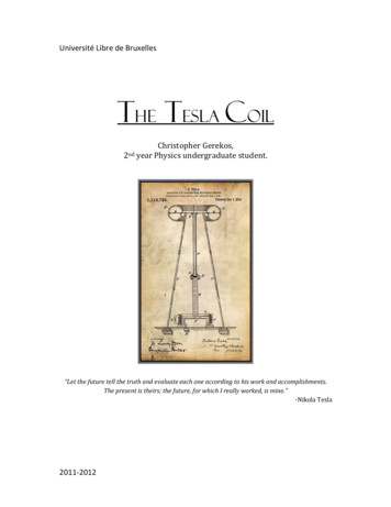
Chapter 2The Zeus ProjectThis Tesla coil was presented to the Printemps des Sciences 2012 science fair and is now at the Expérimentarium de Physique science museum at ULB. It was named Zeus (Ζεύς in ancient Greek or Δίας inmodern Greek) ; in honor of the Greek god, king of the Olympians and known for throwing lightning bolts.It has a power of 225 W, which is quite low compared to the coils built by professionals, which oftensurpass several thousands of Watts. It is nevertheless an appreciable power, given the small budget thatwas allocated.Figure 2.1: The Zeus Coil.The construction of Zeus was not an easy task and almost every component had to be rebuilt at leasttwice. This however allowed me to acquire my first experience in the domain of high voltages, which wasprobably the greatest reward this project gave me.3
4CHAPTER 2. THE ZEUS PROJECTFigure 2.2: Cool beautiful arcs. 1s shutter speed [Photographs: Jean-Louis Colot].
Chapter 3Theory of operationIn this chapter, we will discuss the theory of operation of Tesla coils in a general way. For the moment,let us introduce this short definition:A Tesla coil is a device producing a high frequency current, at a very high voltage but of relatively smallintensity.Basically, it works as a transformer and as a radio antenna, even if it differs radically from these.Figure 3.1: Basic electric schematic of a Tesla coil. [Schematic : Wikipedia]3.1Reminder of the basics3.1.1ResistorA resistor is a component that opposes a flowing current.Every conductor has a certain resistancei If one applies a potential differenceV at the terminals of a resistor, the current I passing through it is given byI VR(3.1) Figure 3.2: Symbol ofa resistor.This formula is know as Ohm’s Law ii . The SI unit of resistance is the Ohm, [Ω].i Exceptii Georgsupraconductors, which have a strictly zero resistance.Simon Ohm : German physicist, 1789-1854.5
6CHAPTER 3. THEORY OF OPERATIONOne can show that the power P (in J/s) dissipated due to a resistance is equal toP V I RI 23.1.2(3.2)CapacitorA capacitor is a component that can store energy in the form of an electric field.Less abstractly, it is composed in its most basic form of two electrodes separatedby a dielectric medium. If there is a potential difference V between those twoelectrodes, charges will accumulates on those electrodes : a charge Q on the positive Figure 3.3: Symbol ofelectrode and an opposite charge Q on the negative one. An electrical field a capacitor.therefore arise between them. If both of the electrodes carry the same amount ofcharge, one can writeQ CVwhere C is the capacity of the capacitor. Its unit is the FaradThe energy E stored in a capacitor (in Joules) is given byE (3.3)iii[F].11QV CV 222(3.4)where one can note that the dependence in the charge Q shows that the energy is indeed the energy ofthe electric field. This corresponds to the amount of work that has to be done to place the charges on theelectrodes.3.1.3InductorAn inductor stores the energy in the form a magnetic field.Every electrical circuit is characterized by a certain inductance. When currentflows within a circuit, it generate a magnetic field B that can be calculated fromMaxwell-Ampere’s lawiv : B µ0 J µ0 ε0 E tFigure 3.4: Symbol ofan inductor(3.5)where E is the electric field and J is the current density. The auto-inductance of a circuit measures itstendency to oppose a change in current : when the current changes, the flux of magnetic field ΦB thatcrosses the circuit changes. That leads to the apparition of an "electromotive force"v E that opposes thischange. It is given by ΦBE (3.6) tThe inductance L of a circuit is thus defined as :V Liii Michael I t(3.7)Faraday : British physicist and chemist, 1791-1867.Clerk Maxwell, Scottish physicist and mathematician, 1831-1879. André-Marie Ampère, French physicist andmathematician, 1755-1836.v This is not properly a force, as the units of E are Volts. The point is that we cannot talk of a potential difference betweentwo points, as the current flows without a material voltage generator.iv James
3.1. REMINDER OF THE BASICS7where I(t) is the current that flows in the circuit and V the electromotive force (emf) that a change ofthis current will provoke. The inductance is measured in henrysvi [H].The energy E (in Joules) stored in an inductor is given byE 1 2LI2(3.8)where the dependence in the current I shows that this energy originates from the magnetic field. Itcorresponds to the work that has to be done against the emf to establish the current in the circuit.3.1.4ImpedanceThe impedance of a component expresses its resistance to an alternating current (i.e. sinusoidal). Thisquantity generalizes the notion of resistance. Indeed, when dealing with alternating current, a componentcan act both on the amplitude and the phase of the signal.Expressions for alternating currentIt is convenient to use the complex plan to represent the impedance. The switching between the two representations is accomplished by using Euler’s formula. Let’s note that the utilization of complex numbersis a simple mathematical trick, as it is understood that only the real part of these quantities is meaningful.We are now given an expression of the general form of the voltage V(t) and current I(t) :V (t) V0 · cos (ωt φV ) I(t) I0 · cos (ωt φI ) noV (t) V0 · Re ej(ωt φV )noI(t) I0 · Re ej(ωt φI )(3.9)(3.10)where V0 and I0 are the respective amplitudes, ω 2πν is the angular speed (assumed identical for bothquantities) and φ are the phases.Definition of impedanceThe impedance, generally noted Z, is formed of a real part, the resistance R, and an imaginary part, thereactance X :Z R jX Z ejθ(cartesian form)(polar form)(3.11)(3.12)where j is the imaginary unit number,i.e. j 2 1, theta arctan(X/R) is the phase difference between 2voltage and current, and Z R X 2 is the euclidean norm of Z in the complex plane.At this point, we can generalize Ohm’s law as the following :V (t) Z · I(t)(3.13)When the component only acts on the amplitude, in other words when X 0, the imaginary partvanishes and we find Z R. We therefore have the behavior of a resistor. The component is then said tobe purely resistive, and the DC version of Ohm’s law (3.1) applies.When the component only acts on the phase of the signal, that is when R 0, the impedance is purelyimaginary. This translates the behavior of "perfect" capacitors and inductors.vi JosephHerny, American physicist, 1797-1878.
8CHAPTER 3. THEORY OF OPERATIONFigure 3.5: The impedance Z plotted in the complex plane. [Diagram : Wikipedia]Impedance formulasWe can give a general formula for the impedance of each type of component.ComponentImpedanceEffect on an alternating signalResistorZ RDiminution of amplitude (current and tension).CapacitorZ 1jCωTension has a π/2 delay over current.InductorZ jLωCurrent has a π/2 delay over tension.These formulas are easily recovered from the differential expressions of these components. For everycombinations of components, one can calculate the phase difference between current and voltage by vectoradding the impedances (for example, in an RC circuit, the phase difference will be less than π/2).Finally, it is good to keep in mind that any real-life component has a non-zero resistance and reactance.Even the simplest circuit, a wire connected to a generator has a capacitance, an inductance and a resistance,however small these might be.3.2LC circuitAn LC circuit is formed with a capacitor C and an inductor L connected in parallel or in series toa sinusoidal signal generator. The understanding of this circuit is at the very basis of the Tesla coilfunctioning, hence the following analysis.The primary and secondary circuits of a Tesla coil are both series LC circuitsvii that are magneticallycoupled to a certain degree. We will therefore only look at the case of the series LC circuit.Figure 3.6: Schematic of a series LC circuit.Using Kirchoff’s law for current, we obtain that the current in the inductor and the current in thecapacitor is identical. We now use Kirchoff’s law for voltage, which sates that the sum of the voltagesvii Of course, they’re actually RLC circuits, which, we’ll talk about later, as all the components and wires have a certainresistance. However, materials used as well as the section of the conductors keep this resistance negligible. We can thereforeconsider in first approximation that the real circuits behave like LC circuits.
3.2. LC CIRCUIT9across the components along a closed loop is zero, to get the following equation :Vgen (t) VL (t) VC (t)(3.14)For the inductor, we use the equality (3.7) and express the time derivative of current in terms of thecharge by I dQdt . We findVL (t)dIdtd2 Q L 2dt L(3.15)(3.16)Now for the capacitor, we isolate the charge Q in the relation (3.3) and getVC (t) 1Q(t)C(3.17)Plugging these two results in (3.14), we obtain :Vgen (t) LQ̈ 1QC(3.18)This equation describes an (undamped) harmonic oscillator with periodic driving, just like a spring-masssystem! The inductor is assimilated to the "mass" of the oscillator : a circuit of great inductance will havea lot of "inertia". The "spring constant" is associated with the inverse of the capacitance C 1 (this is thereason why C 1 is seldom called the "elastance").Homogeneous solutionThe homogeneous equation, i.e. without independent term (representing the generator, in this case) is thefollowing :1LQ̈ Q 0(3.19)CThis equation corresponds to a real situation: the capacitor holds a certain charge and we let thesystem evolute freely. The mechanical analogy with the spring-mass system correspond to an initial statewhere the spring is tense and when no other force interactsviiiWe find the solution to equation (3.19) with the characteristic polynomial method. We obtain a sumof complex exponentials, which is of course an oscillating solution as expected.Q(t) K1 ejωt K2 e jωt(3.20) where we noted ω 1/ LC.Setting Q(0) Q0 and Q̇(0) I(0) 0, which indeed corresponds to the initial condition where thecapacitor is fully loaded and no current initially flows in the inductor, we getK1K2 Q0 22(3.21)We now take the real part of Q(t), but thanks to (3.21), the solution is already real : Q(t) Q0 cos (ωt) Q0 cosviii Equationt LC (3.19) has of course the trivial solution Q(t) 0 t, but we won’t consider it here.(3.22)
10CHAPTER 3. THEORY OF OPERATIONWe now find the current flows through the inductor by time-derivating the above expression for thecharge stored in the capacitor : Q0tI(t) (3.23)sin LCLCThe next figures give a good intuition of what actually happens in the circuit. We look at the voltageV (t) between the leads of the capacitor as well as the current I(t) running into the inductor (which is thesame in the entire circuit, as previously stated). For convenience, we put all the constants Q0 , L, and Cto unity.Figure 3.7: LC circuits with voltmeter and ammeterFigure 3.8: Plot of tension in current versus time.Step 0: At the initial instant, the capacitor is fully charged and no current flows. Immediately after,the capacitor begins to discharge: the voltage decreases as a current gradually appears in the circuit.Step 1: When the capacitor is totally discharged, the voltages at its leads is zero. If there was noinductance, things would stop right here. However, the inductor opposes this brutal drop of current bygenerating an electromotive force that will keep the current goingix . In this way, the current graduallydecreases (instead of stopping abruptly) and recharges the capacitor on the way (with an opposite polarity).Step 2: The capacitor is fully charged again, with opposite polarity now, and the current has fallen tozero. However the charges stored in the capacitor are wanting to neutralize themselvesx : a current willreappear while the voltage is decreasing again.Step 3: The capacitor is "empty" again (zero voltage), but the inductor prevents the current fromstopping abruptly. This current will now recharge the capacitor with reversed polarity .Step 4: . and the situation is exactly like it was at the initial instant.We have already noted at this point that the system naturally oscillates at a certain resonant angular1speed ω LC, which is univoquely determined by the inductance and the capacitance of the circuit.ix Letus remember the mechanical analogy :inductance gives "inertia" to the circuits.like a tense spring wants to recover its neutral shape.x Just
3.2. LC CIRCUIT11General solution.We reconsider equation (3.18) with its independent term, where we explicitly state the fact that thegenerator produces a sinusoidal voltage of amplitude, say, V0 and of pulsation Ω:LQ̈ 1Q V0 sin (Ωt)C(3.24)We will find a specific solution to obtain the general solutionIf ω 6 Ω. We make an educated guess about a specific solution Qp by stating it has the following form:Qp A sin (Ωt ϕ), with amplitude A and phase ϕ to be determined. We derivate this guessed solutiontwice and inject it straight into our starting equation (3.24) : 1 Ω2 L sin (Ωt ϕ) V0 sin (Ωt)(3.25)ACEquating amplitude and phase into the two parts of this equality, we deduce :(V0V0A 1/C Ω2 L L(ω 2 Ω2 )ϕ 0(3.26)The specific solution is therefore :Qp (t) V0sin (Ωt)L(ω 2 Ω2 )(3.27)We can now find the general solution by adding the specific solution to the homogeneous solution(3.20).V0sin (Ωt)Q(t) K̃1 cos (ωt) K̃2 sin (ωt) (3.28)L(ω 2 Ω2 )The current is :I(t) ω K̃2 cos (ωt) ω K̃1 sin (ωt) V0 Ωcos (Ωt)L(ω 2 Ω2 )(3.29)where the constants K̃1 and K̃2 can be found in terms of the initial conditions.We see that we still have sinusoidal functions. If ω is close to Ω, the oscillations will be of greatamplitude because of the "new" term, but will remain bounded. When ω is very far from Ω, the new termbecomes negligible.If ω Ω. Here, the specific solution is more difficult to find. Let us rewrite (3.24) in a more convenientway :V0 jωtQ̈ ω 2 Q (e e jωt )(3.30)2LjHere, we’ll guess that the specific solution has the following form ; Qp (t) (A B t)ejωt (A B t)e jωt . This makes sense physically, as we expect the voltage and current to have amplitudes thatktincrease with time. We rewrite it in a more condensed manner kt : Qp (t) (A Bt)e with k jω. The2second time-derivative yields Q̈p (t) k (A Bt) 2kB e . We plug thses expression in (3.30) in orderto refine them : 2 V0 kt(k ω 2 )(A Bt) 2kB ekt e(3.31)2Lj
12CHAPTER 3. THEORY OF OPERATIONWe compare the two side of the equality as before.When k jω, we find2jωB ejωt B V0 jωte2LjV04Lω(3.32)(3.33)When k jω,V0 jωte(3.34)2LjV0B (3.35)4LωWe have therefore found that B B B. And as we have found no constraints on the A’s, we setthem equal to zero. We have now obtained our specific solution : 2jωB e jωt Btejωt Bte jωt V0 t jωte e jωt 4LωV0 t cos (ωt)2LωThe general solution for the voltage is therefore :Qp (t)Q(t) K̃1 cos (ωt) K̃2 sin (ωt) V0 tcos (ωt)2Lω(3.36)(3.37)(3.38)(3.39)and the current is :I(t) V0V0 ωtsin (ωt)ω K̃2 cos (ωt) ω K̃1 sin (ωt) 2Lω2Lω(3.40)where the constants K̃1 and K̃2 can be found in terms of the initial conditions.In this case, we see we’re no longer dealing with simple oscillations. The last term of the solutionindicates that the amplitude of the voltage and current will increase at each cycle, and grow to infinity ast .3.2.1ImpedanceWe’ll have to calculate the impedance of the LC circuits inside the Tesla coil. Let us recall that thecapacitor and the inductor are connected in series on the generator. The total impedance is thereforeequal to the sum of the impedances of each component.Z ZC ZL1 jLωjCωω 2 LC 1jωC(3.41)(3.42)(3.43)We see that, at the resonant pulsation, ω 2 LC 1 and the impedance vanishes. A series LC circuitplaced in series on a wire will therefore act as a band-pass filter. Similarly, a parallel LC circuit will act asa band-stop filter when connected in series on the wire [2]. There are many other possibilities for filters,but this is not within the scope of the present document.
3.2. LC CIRCUIT3.2.213Resonant frequencyIn our analysis of the LC circuit, we found that the oscillations of current and voltage naturally occurred ata precise angular speed, univoquely determined by the capacitance and inductance of the circuit. Withoutother effects, oscillations of current and voltage will always take place at this angular speed.ωres 1LC(3.44)It is called the resonant angular speed. We can check that it is dimensionally coherent (its units are s 1 ).It is however much more common to talk about resonant frequency, which is just a rescale of the angularspeed :1 fres (3.45)2π LCIt is no less important to observe that, at the resonant angular speed, the respective reactive parts ofan inductor and a capacitor are equal (in absolute value) : LL XLres XCres (3.46)LCCWhen there is a sinusoidal signal generator, we also saw that if its frequency is equal to the resonantfrequency of the circuit it drives, current and voltage have ever-increasing amplitudes. Of course, thisdoesn’t happen if they are different (the oscillation remain bounded).Figure 3.9: Amplitude of the current plotted against the driving frequency (all constants normalized). [Diagram :Wikipedia]At low driving frequencies, the impedance is mainly capacitive as the reactance of a capacitor is greaterat low frequencies. At high frequencies, the impedance is mainly inductive. At the resonant frequency,it vanishes, hence the asymptotic behavior of the current. However, in a real circuit, where resistance isnon-zero, the width and height of the "spike" plotted her above are determined by the Q factor, whichwe’ll talk about later.The fact that driving an (R)LC circuit at its resonant frequency causes a dramatic increase of voltageand current is crucial for a Tesla coil. But it can also be potentially harmful for the transformer feedingthe primary circuit. These practical considerations will be addressed in the next chapter.3.2.3RLC circuitAn RLC circuit is an LC circuit on which a resistance was added. This kind of circuit can take multipleforms. We won’t analyze it here, but we’ll give its major characteristicsxi .xi Athorough treatment is given in Appendix C.
14CHAPTER 3. THEORY OF OPERATIONFigure 3.11: Amplitude of the current vs driving frequencyfor an RLC circuit (all constants normalized). [Diagram: Wikipedia]Figure 3.10: Schematic of a series RLC circuit.The resistance (VR (t) RQ0 (t)) dissipates the circuits energy as heat, whatever the direction of thecurrent. It therefore acts like a friction force. Without a generator, current and voltage will graduallydecrease as they oscillate (the circuit is said to be underdamped ) or, if the resistance is high enough, nooscillation will take place (overdamped circuit).In the underdamped case, the graph of current or voltage is a sine wave whose amplitude decreasesexponentially with time. If there is a driving force, the resistance will prevent the system from havingoscillations of ever-increasing amplitude. And finally, instead of a spike, the RLC circuit has a bandwidth.One can show that the resonant frequency of a RLC circuit is the same as the LC circuit [3][4]:fres 1 2π LC(3.47)To find its impedance, we just have to add the value of the resistance R to (3.43). While the LC circuithad a purely imaginary impedance, the RLC circuit has a real part as well : 1Z R j ωL (3.48)ωCQ factor.The Q factor (for quality) is a dimensionless quantity which characterizes every RLC circuit, or moregenerally, every damped oscillator. It measures the narrowness of the bandwidth : a large Q factordenotes a spiky bandwidthxii .More precisely, the Q factor represents the ratio between the energy stored in the circuit and the energydissipated during the oscillations [5]. This can also be expressed in power terms [6] :Q PstoredPdissipatedXR XI 2RI 2where X is the reactance of the inductor/capacitor at the resonant frequency.For a RLC circuit, this becomes, using (3.45) :r1 LQ R Cxii In(3.49)(3.50)(3.51)the stricter sense, the Q factor of a LC circuit is infinite, but the quantity is not really meaningful in this case.
3.3. TESLA COIL OPERATION15One can also give a definition of the bandwidth f as a function of the Q factor [6] : f fresQ(3.52)It is then clear why this quantity is called the quality factor : an RLC circuit of "great quality" isstrongly underdamped and will therefore dissipate very little energy per cycle [6]. Moreover, its bandwidthwill be very narrow, which is desirable, for example, in a radio receiver.Figure 3.12: Effect of the Q factor on the bandwidth size. [Diagram : All About Circuits]3.3Tesla coil operationThis is where the fun begins.This section shall cover the complete theory of operation of a conventional Tesla coil. We will considerthat the primary and secondary circuits are RLC circuits with low resistance, which accords with realityxiii .We consider a slightly modified version of figure 3.1 to illustrate our explanations. For the aforementioned reasons, internal resistance of the component aren’t represented. We will also replace thecurrent-limited transformer. This has no impact regarding pure theoryxiv .Note that some parts of the secondary circuit are drawn in dotted lines. This is because they are notdirectly visible on the apparatus. Regarding the secondary capacitor, we’ll see that its capacity is actuallydistributed, the top load only being "one plate" of this capacitor. Regarding the secondary spark gap, itis shown in the schematic as a way to represent where the arcs will take place.3.3.1Description of a cycleThis is perhaps the most important section. In order to make it lighter, specific details of the individualcomponents won’t be discussed until Chapter 4.xiii Amore rigorous analysis is given in Appendix D.implications of the choice of the transformer/generator are discussed in the next chapter.xiv Practical
16CHAPTER 3. THEORY OF OPERATIONFigure 3.13: Schematic of the basic features of a Tesla coil.Charging.This first step of the cycle is the charging of the primary capacitor by the generator. We’ll suppose itsfrequency to be 50 Hz.Because the generator is current-limited, the capacity of the capacitor must be carefully chosen so itwill be fully charged in exactly 1/100 seconds. Indeed, the voltage of the generator changes twice a period,and at the next cycle, it will re-charge the capacitor with opposite polarity, which changes absolutelynothing about the operation of the Tesla coil.Figure 3.14: The generator charges the primary caps.Oscillations.When the capacitor is fully charged, the spark gap fires and therefore closes the primary circuit. Knowingthe intensity of the breakdown electric field of air, the width of the spark gap must be set so that it firesexactly when the the voltage across the capacitor reaches its peak value. The role of the generator endshere xv .We now have a fully loaded capacitor in an LC circuit! Current and voltage will thus oscillate at thecircuits resonant frequency, as it was demonstrated in equations (3.22) and (3.23). This frequency is veryhigh compared to the mains frequency, generally between 50 and 400 kHz xvi
Nikola Tesla was born the 10th of July 1856 in a Serbian village of the Austrian Empire (in today’s Croatia)anddiedthe7th ofJanuary1943intheUnitedStates[1]. It is not an exaggeration to say he was a visionary who changed the world. With his works on alternative current, including many