WIXLIB

Chapter 1IntroductionThe interest in the freely available statistical programming language and software environment R (R Core Team, 2020) is soaring. By the time we wrotefirst drafts for this project, more than 11000 add-ons (many of them providingcutting-edge methods) were made available on the Comprehensive R ArchiveNetwork (CRAN), an extensive network of FTP servers around the world thatstore identical and up-to-date versions of R code and its documentation. R dominates other (commercial) software for statistical computing in most fields ofresearch in applied statistics. The benefits of it being freely available, opensource and having a large and constantly growing community of users that contribute to CRAN render R more and more appealing for empirical economistsand econometricians alike.A striking advantage of using R in econometrics is that it enables students toexplicitly document their analysis step-by-step such that it is easy to update andto expand. This allows to re-use code for similar applications with different data.Furthermore, R programs are fully reproducible, which makes it straightforwardfor others to comprehend and validate results.Over the recent years, R has thus become an integral part of the curricula ofeconometrics classes we teach at the University of Duisburg-Essen. In somesense, learning to code is comparable to learning a foreign language and continuous practice is essential for the learning success. Needless to say, presentingbare R code on slides does not encourage the students to engage with hands-onexperience on their own. This is why R is crucial. As for accompanying literature, there are some excellent books that deal with R and its applications toeconometrics, e.g., Kleiber and Zeileis (2008). However, such sources may besomewhat beyond the scope of undergraduate students in economics having littleunderstanding of econometric methods and barely any experience in programming at all. Consequently, we started to compile a collection of reproduciblereports for use in class. These reports provide guidance on how to implementselected applications from the textbook Introduction to Econometrics (Stock11

12CHAPTER 1. INTRODUCTIONand Watson, 2015) which serves as a basis for the lecture and the accompanying tutorials. This process was facilitated considerably by knitr (Xie, 2020b)and R markdown (Allaire et al., 2020). In conjunction, both R packages providepowerful functionalities for dynamic report generation which allow to seamlesslycombine pure text, LaTeX, R code and its output in a variety of formats, including PDF and HTML. Moreover, writing and distributing reproducible reportsfor use in academia has been enriched tremendously by the bookdown package(Xie, 2020a) which has become our main tool for this project. bookdown buildson top of R markdown and allows to create appealing HTML pages like this one,among other things. Being inspired by Using R for Introductory Econometrics(Heiss, 2016)1 and with this powerful toolkit at hand we wrote up our own empirical companion to Stock and Watson (2015). The result, which you startedto look at, is Introduction to Econometrics with R.Similarly to the book by Heiss (2016), this project is neither a comprehensiveeconometrics textbook nor is it intended to be a general introduction to R. Wefeel that Stock and Watson do a great job at explaining the intuition and theoryof econometrics, and at any rate better than we could in yet another introductory textbook! Introduction to Econometrics with R is best described as aninteractive script in the style of a reproducible research report which aims toprovide students with a platform-independent e-learning arrangement by seamlessly intertwining theoretical core knowledge and empirical skills in undergraduate econometrics. Of course, the focus is on empirical applications with R. Weleave out derivations and proofs wherever we can. Our goal is to enable studentsnot only to learn how results of case studies can be replicated with R but wealso intend to strengthen their ability in using the newly acquired skills in otherempirical applications — immediately within Introduction to Econometrics withR.To realize this, each chapter contains interactive R programming exercises.These exercises are used as supplements to code chunks that display how previously discussed techniques can be implemented within R. They are generatedusing the DataCamp light widget and are backed by an R session which is maintained on DataCamp’s servers. You may play around with the example exercisepresented below.As you can see above, the widget consists of two tabs. script.R mimics an .Rfile, a file format that is commonly used for storing R code. Lines starting witha # are commented out, that is, they are not recognized as code. Furthermore,script.R works like an exercise sheet where you may write down the solutionyou come up with. If you hit the button Run, the code will be executed, submission correctness tests are run and you will be notified whether your approach iscorrect. If it is not correct, you will receive feedback suggesting improvementsor hints. The other tab, R Console, is a fully functional R console that can beused for trying out solutions to exercises before submitting them. Of course1 Heiss (2016) builds on the popular Introductory Econometrics (Wooldridge, 2016) anddemonstrates how to replicate the applications discussed therein using R.

1.1. COLOPHON13you may submit (almost any) R code and use the console to play around andexplore. Simply type a command and hit the Enter key on your keyboard.Looking at the widget above, you will notice that there is a in the right panel(in the console). This symbol is called “prompt” and indicates that the usercan enter code that will be executed. To avoid confusion, we will not show thissymbol in this book. Output produced by R code is commented out with # .Most commonly we display R code together with the generated output in codechunks. As an example, consider the following line of code presented in chunkbelow. It tells R to compute the number of packages available on CRAN. Thecode chunk is followed by the output produced.# check the number of R packages available on CRANnrow(available.packages(repos "http://cran.us.r-project.org"))# [1] 16272Each code chunk is equipped with a button on the outer right hand side whichcopies the code to your clipboard. This makes it convenient to work with largercode segments in your version of R/RStudio or in the widgets presented throughout the book. In the widget above, you may click on R Console and typenrow(available.packages(repos "http://cran.us.r-project.org"))(the command from the code chunk above) and execute it by hitting Enter onyour keyboard.2Note that some lines in the widget are out-commented which ask you to assigna numeric value to a variable and then to print the variable’s content to theconsole. You may enter your solution approach to script.R and hit the buttonRun in order to get the feedback described further above. In case you do notknow how to solve this sample exercise (don’t panic, that is probably why youare reading this), a click on Hint will provide you with some advice. If youstill can’t find a solution, a click on Solution will provide you with another tab,Solution.R which contains sample solution code. It will often be the case thatexercises can be solved in many different ways and Solution.R presents whatwe consider as comprehensible and idiomatic.1.1ColophonThis book was build with:# - Session info ------------# setting value# version R version 4.0.2 (2020-06-22)2 The R session is initialized by clicking into the widget. This might take a few seconds.Just wait for the indicator next to the button Run to turn green.

14CHAPTER 1. INTRODUCTION# osmacOS Catalina 10.15.4# systemx86 64, darwin19.5.0# uiunknown# language (EN)# collate en US.UTF-8# ctypeen US.UTF-8# tzEurope/Berlin# date2020-09-15# # - Packages ----------------# package* versiondatelib source# abind1.4-52016-07-21 [1] CRAN (R 4.0.2)# AER1.2-92020-02-06 [1] CRAN (R 4.0.0)# askpass1.12019-01-13 [1] CRAN (R 4.0.0)# assertthat0.2.12019-03-21 [1] CRAN (R 4.0.0)# backports1.1.82020-06-17 [1] CRAN (R 4.0.0)# base64enc0.1-32015-07-28 [1] CRAN (R 4.0.0)# bdsmatrix1.3-42020-01-13 [1] CRAN (R 4.0.0)# BH1.72.0-32020-01-08 [1] CRAN (R 4.0.2)# bibtex0.4.2.22020-01-02 [1] CRAN (R 4.0.0)# bitops1.0-62013-08-17 [1] CRAN (R 4.0.0)# blob1.2.12020-01-20 [1] CRAN (R 4.0.0)# bookdown0.202020-06-23 [1] CRAN (R 4.0.0)# boot1.3-252020-04-26 [2] CRAN (R 4.0.2)# broom0.7.02020-07-09 [1] CRAN (R 4.0.2)# callr3.4.32020-03-28 [1] CRAN (R 4.0.0)# car3.0-82020-05-21 [1] CRAN (R 4.0.0)# carData3.0-42020-05-22 [1] CRAN (R 4.0.0)# cellranger1.1.02016-07-27 [1] CRAN (R 4.0.0)# cli2.0.22020-02-28 [1] CRAN (R 4.0.0)# clipr0.7.02019-07-23 [1] CRAN (R 4.0.0)# colorspace1.4-12019-03-18 [1] CRAN (R 4.0.0)# conquer1.0.12020-05-06 [1] CRAN (R 4.0.2)# crayon1.3.42017-09-16 [1] CRAN (R 4.0.0)# cubature2.0.4.12020-07-06 [1] CRAN (R 4.0.2)# curl4.32019-12-02 [1] CRAN (R 4.0.0)# data.table1.12.82019-12-09 [1] CRAN (R 4.0.0)# DBI1.1.02019-12-15 [1] CRAN (R 4.0.0)# dbplyr1.4.42020-05-27 [1] CRAN (R 4.0.0)# desc1.2.02018-05-01 [1] CRAN (R 4.0.0)# digest0.6.252020-02-23 [1] CRAN (R 4.0.0)# dplyr1.0.02020-05-29 [1] CRAN (R 4.0.0)# dynlm0.3-62019-01-06 [1] CRAN (R 4.0.2)# ellipsis0.3.12020-05-15 [1] CRAN (R 4.0.0)# evaluate0.142019-05-28 [1] CRAN (R 4.0.0)# fansi0.4.12020-01-08 [1] CRAN (R 4.0.0)

1.1. COLOPHON# # # # # # # # # # # # # # # # # # # # # # # # # # # # # # # # # # # # # # # # # # # # # # ][1][1][1][2][2][1][1][1][2][1][1][1][1][1][1]CRAN (R 4.0.0)CRAN (R 4.0.2)CRAN (R 4.0.2)CRAN (R 4.0.2)CRAN (R 4.0.0)CRAN (R 4.0.2)CRAN (R 4.0.0)CRAN (R 4.0.2)CRAN (R 4.0.0)CRAN (R 4.0.0)CRAN (R 4.0.0)CRAN (R 4.0.0)CRAN (R 4.0.2)CRAN (R 4.0.0)CRAN (R 4.0.0)CRAN (R 4.0.0)CRAN (R 4.0.0)CRAN (R 4.0.0)CRAN (R 4.0.2)CRAN (R 4.0.0)Github (mca91/itewrpkg@bf5448c)CRAN (R 4.0.0)CRAN (R 4.0.2)CRAN (R 4.0.0)CRAN (R 4.0.0)CRAN (R 4.0.2)CRAN (R 4.0.0)CRAN (R 4.0.0)CRAN (R 4.0.2)CRAN (R 4.0.0)CRAN (R 4.0.0)CRAN (R 4.0.0)CRAN (R 4.0.0)CRAN (R 4.0.0)CRAN (R 4.0.2)CRAN (R 4.0.2)CRAN (R 4.0.0)CRAN (R 4.0.2)CRAN (R 4.0.0)CRAN (R 4.0.2)CRAN (R 4.0.0)CRAN (R 4.0.0)CRAN (R 4.0.0)CRAN (R 4.0.0)CRAN (R 4.0.0)CRAN (R 4.0.2)

16# # # # # # # # # # # # # # # # # # # # # # # # # # # # # # # # # # # # # # # # # # # # # # CHAPTER 1. 0.0)4.0.0)

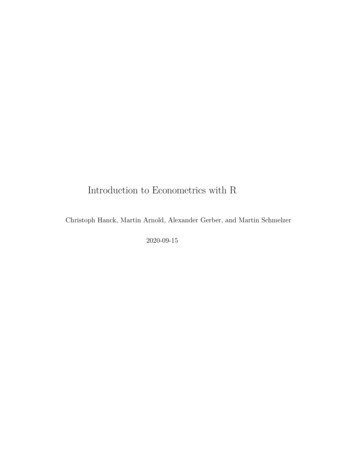
1.2. A VERY SHORT INTRODUCTION TO R AND RSTUDIO# SparseM1.782019-12-13 [1] CRAN# spatial7.3-122020-04-26 [2] CRAN# stabledist0.7-12016-09-12 [1] CRAN# stargazer5.2.22018-05-30 [1] CRAN# statmod1.4.342020-02-17 [1] CRAN# stringi1.4.62020-02-17 [1] CRAN# stringr1.4.02019-02-10 [1] CRAN# strucchange1.5-22019-10-12 [1] CRAN# survival3.2-32020-06-13 [2] CRAN# sys3.42020-07-23 [1] CRAN# testthat2.3.22020-03-02 [1] CRAN# tibble3.0.32020-07-10 [1] CRAN# tidyr1.1.02020-05-20 [1] CRAN# tidyselect1.1.02020-05-11 [1] CRAN# tidyverse1.3.02019-11-21 [1] CRAN# timeDate3043.1022018-02-21 [1] CRAN# timeSeries3062.1002020-01-24 [1] CRAN# tinytex0.252020-07-24 [1] CRAN# TTR0.23-62019-12-15 [1] CRAN# urca1.3-02016-09-06 [1] CRAN# utf81.1.42018-05-24 [1] CRAN# vars1.5-32018-08-06 [1] CRAN# vctrs0.3.22020-07-15 [1] CRAN# viridisLite0.3.02018-02-01 [1] CRAN# whisker0.42019-08-28 [1] CRAN# withr2.2.02020-04-20 [1] CRAN# xfun0.162020-07-24 [1] CRAN# xml21.3.22020-04-23 [1] CRAN# xts0.12-02020-01-19 [1] CRAN# yaml2.2.12020-02-01 [1] CRAN# zip2.0.42019-09-01 [1] CRAN# zoo1.8-82020-05-02 [1] CRAN# # [1] /usr/local/lib/R/4.0/site-library# [2] /usr/local/Cellar/r/4.0.2 0)4.0.0)4.0.0)4.0.0)4.0.0)A Very Short Introduction to R and RStudioR BasicsAs mentioned before, this book is not intended to be an introduction to R buta guide on how to use its capabilities for applications commonly encountered inundergraduate econometrics. Those having basic knowledge in R programmingwill feel comfortable starting with Chapter 2. This section, however, is meant

18CHAPTER 1. INTRODUCTIONFigure 1.1: RStudio: the four panesfor those who have not worked with R or RStudio before. If you at least knowhow to create objects and call functions, you can skip it. If you would like torefresh your skills or get a feeling for how to work with RStudio, keep reading.First of all, start RStudio and open a new R script by selecting File, New File,R Script. In the editor pane, type1 1and click on the button labeled Run in the top right corner of the editor. Bydoing so, your line of code is sent to the console and the result of this operationshould be displayed right underneath it. As you can see, R works just like acalculator. You can do all arithmetic calculations by using the correspondingoperator ( , -, *, / or ). If you are not sure what the last operator does, tryit out and check the results.VectorsR is of course more sophisticated than that. We can work with variables or,more generally, objects. Objects are defined by using the assignment operator -. To create a variable named x which contains the value 10 type x - 10and click the button Run yet again. The new variable should have appeared inthe environment pane on the top right. The console however did not show anyresults, because our line of code did not contain any call that creates output.When you now type x in the console and hit return, you ask R to show you thevalue of x and the corresponding value should be printed in the console.x is a scalar, a vector of length 1. You can easily create longer vectors by usingthe function c() (c is for “concatenate” or “combine”). To create a vector ycontaining the numbers 1 to 5 and print it, do the following.

1.2. A VERY SHORT INTRODUCTION TO R AND RSTUDIO19y - c(1, 2, 3, 4, 5)y# [1] 1 2 3 4 5You can also create a vector of letters or words. For now just remember thatcharacters have to be surrounded by quotes, else they will be parsed as objectnames.hello - c("Hello", "World")Here we have created a vector of length 2 containing the words Hello and World.Do not forget to save your script! To do so, select File, Save.FunctionsYou have seen the function c() that can be used to combine objects. In general,all function calls look the same: a function name is always followed by roundparentheses. Sometimes, the parentheses include arguments.Here are two simple examples.# generate the vector z z - seq(from 1, to 5, by 1)# compute the mean of the enries in z mean(z)# [1] 3In the first line we use a function called seq() to create the exact same vectoras we did in the previous section, calling it z. The function takes on the arguments from, to and by which should be self-explanatory. The function mean()computes the arithmetic mean of its argument x. Since we pass the vector z asthe argument x, the result is 3!If you are not sure which arguments a function expects, you may consult thefunction’s documentation. Let’s say we are not sure how the arguments requiredfor seq() work. We then type ?seq in the console. By hitting return thedocumentation page for that function pops up in the lower right pane of RStudio.In there, the section Arguments holds the information we seek. On the bottomof almost every help page you find examples on how to use the correspondingfunctions. This is very helpful for beginners and we recommend to look out forthose.Of course, all of the commands presented above also work in interactive widgetsthrou

ature, there are some excellent books that deal with Rand its applications to econometrics, e.g., Kleiber and Zeileis (2008). However, such sources may be . ing PDF and HTML. Moreover, writing and distributing reproducible reports .