WIXLIB

Gibbs and Metropolis sampling (MCMC methods)and relations of Gibbs to EMLecture Outline1. Gibbs the algorithm a bivariate example an elementary convergence proof for a (discrete) bivariate case more than two variables a counter example.2. EM – again EM as a maximization/maximization method Gibbs as a variation of Generalized EM3. Generating a Random Variable. Continuous r.v.s and an exact method based on transforming the cdf. The “accept/reject” algorithm. The Metropolis Algorithm1

Gibbs SamplingWe have a joint densityf(x, y1, , yk)and we are interested, say, in some features of the marginal densityf(x) f(x, y1, , yk) dy1, dy2, , dyk.For instance, suppose that we are interested in the averageE[X] x f(x)dx.If we can sample from the marginal distribution, thenlimm 1nn X i E[X]i 1without using f(x) explicitly in integration. Similar reasoning applies toany other characteristic of the statistical model, i.e., of the population.2

The Gibbs Algorithm for computing this average.Assume we can sample the k 1-many univariate conditional densities:f(X y1, , yk)f(Y1 x, y2, , yk)f(Y2 x, y1, y3, , yk) f(Yk x, y1, y3, , yk-1).Choose, arbitrarily, k initial values: Y1 y10 , Y2 y 02 , ., Yk y 0k .Create:00x1 by a draw from f(X y1 , , y k )y11 by a draw from f(Y1 x1 , y 02 , , y 0k )y12 by a draw from f(Y2 x1 , y11, y 30 , y 0k ) y1k by a draw from f(Yk x1 , y11, , y1k 1 ).3

This constitutes one Gibbs “pass” through the k 1 conditional distributions,yielding values:( x1 , y11, y12 , ., y1k ).Iterate the sampling to form the second “pass”( x 2 , y12 , y 22 , ., y 2k ).Theorem: (under general conditions)The distribution of x n converges to F(x) as n .Thus, we may take the last n X-values after many Gibbs passes:1nm ni X i mE[X]or take just the last value, xini of n-many sequences of Gibbs passesnnE[X](i 1, n)1nto solve for the average, x f(x)dx. Xi i i i4

A bivariate example of the Gibbs Sampler.Example: Let X and Y have similar truncated conditional exponentialdistributions:f(X y) ye-yx for 0 X bf(Y x) xe-xy for 0 Y bwhere b is a known, positive constant.Though it is not convenient to calculate, the marginal density f(X) isreadily simulated by Gibbs sampling from these (truncated) exponentials.Below is a histogram for X, b 5.0, using a sample of 500 terminalobservations with 15 Gibbs’ passes per trial, xini (i 1, , 500, ni 15)(from Casella and George, 1992).5

Histogram for X, b 5.0, using a sample of 500 terminal observations with 15 Gibbs’ passes per trial,nxi i(i 1, , 500, ni 15). Taken from (Casella and George, 1992).6

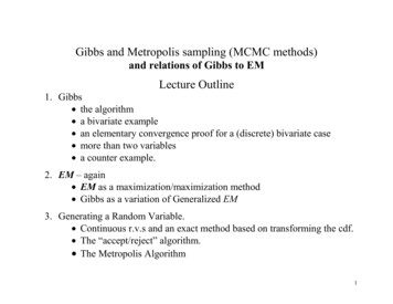
Here is an alternative way to compute the marginal f(X) using the sameGibbs Sampler.Recall the law of conditional expectations (assuming E[X] exists):E[ E[X Y] ] E[X]ThusE[f(x Y)] f(x y)f(y)dy f(x).Now, use the fact that the Gibbs sampler gives us a simulation of themarginal density f(Y) using the penultimate values (for Y) in each Gibbs’n 1yi i (i 1, 500; ni 15).pass, above:Calculate f(x yini 1), which by assumption is feasible.Then note that:f(x) 1nnn 1 f(x yi i )i i7

The solid line graphs the alternative Gibbs Sampler estimate of the marginal f(x) from ethsame sequence of 500 Gibbs’ passes, using f(x y)f(y)dy f(x). The dashed-line is theexact solution. Taken from (Casella and George, 1992).8

An elementary proof of convergence in the case of 2 x 2 Bernoulli dataLet (X,Y) be a bivariate variable, marginally, each is BernoulliX01 p1 p2 Y p p4 1 30where pi 0, pi 1, marginallyP(X 0) p1 p3 and P(X 1) p2 p4P(Y 0) p1 p2 and P(Y 1) p3 p4.9

P(Y x):The conditional probabilities P(X y) and P(Y x) are evident:X012 p p 2 4p4 p p 2 4 p 0 p 1p 1 3Y p31 p p 1 3P(X y):pX0p 0 p 1p 1 2Y p31 p p 3 412 p p 1 2p4 p p 3 4 p10

Suppose (for illustration) that we want to generate the marginaldistribution of X by the Gibbs Sampler, using the sequence of iterationsof draws between the two conditional probabilites P(X y) and P(Y x).That is, we are interested in the sequence xi : i 1, created from thestarting value y 0 0 or y 0 1.Note that:P( X n 0 xi : i 1, , n-1) P( X n 0 x n 1) the Markov property P( X n 0 y n 1 0) P(Y n 1 0 x n 1) P( X n 0 y n 1 1) P(Y n 1 1 x n 1)11

Thus, we have the four (positive) transition probabilities:P( X n j x n 1 i) pij 0, with i j pij 1 (i, j 0, 1).With the transition probabilities positive, it is an (old) ergodic theoremthat, P( X n ) converges to a (unique) stationary distribution, independentof the starting value ( y 0 ).Next, we confirm the easy fact that the marginal distribution P(X) is thatsame distinguished stationary point of this Markov process.12

P( X n 0) P( X n 0 x n 1 0) P( X n 1 0) P( X n 0 x n 1 1) P( X n 1 1)P( X n 0 y n 1 0) P(Y n 1 0 x n 1 0) P( X n 1 0) P( X n 0 y n 1 1) P(Y n 1 1 x n 1 0) P( X n 1 0) P( X n 0 y n 1 0) P(Y n 1 0 x n 1 1) P( X n 1 1) P( X n 0 y n 1 1) P(Y n 1 1 x n 1 1) P( X n 1 1) EP [EP [ X n 0 EP [ X n 0 ] P( X n 0) .X n 1] ]13

The Ergodic Theorem:Definitions: A Markov chain, X0, X1, . satisfiesP(Xn xi: i 1, , n-1) P(Xn xn-1) The distribution F(x), with density f(x), for a Markov chain isstationary (or invariant) if A f(x) dx P(Xn A xn-1) f(x) dx. The Markov chain is irreducible if each set with positive Pprobability is visited at some point (almost surely).14

An irreducible Markov chain is recurrent if, for each set Ahaving positive P-probability, with positive P-probability thechain visits A infinitely often. A Markov chain is periodic if for some integer k 1, there is apartition into k sets {A1, , Ak} such thatP(Xn 1 Aj 1 xn Aj) 1 for all j 1, , k-1 (mod k). Thatis, the chain cycles through the partition.Otherwise, the chain is aperiodic.15

Theorem: If the Markov chain X0, X1, . is irreducible with aninvariant probability distribution F(x) then:1. the Markov chain is recurrent2. F is the unique invariant distributionIf the chain is aperiodic, then for F-almost all x0, both3. limn supA P(Xn A X0 x0 ) – A f(x) dx 0And for any function h with h(x) dx ,4.limn 1nn h( X i ) h(x) f(x) dx ( EF[h(x)] ),i iThat is, the time average of h(X) equals its state-average, a.e. F.16

A (now-familiar) puzzle.Example (continued): Let X and Y have similar conditional exponentialdistributions:f(X y) ye-yx for 0 Xf(Y x) xe-xy for 0 YTo solve for the marginal density f(X) use Gibbs sampling from theseexponential distributions. The resulting sequence does not converge!Question: Why does this happen?Answer: (Hint: Recall HW #1, problem 2.) Let θ be the statisticalparameter for X with f(X θ) the exponential model. What “prior”density for θ yields the posterior f(θ x) xe-xθ?Then, what is the “prior” expectation for X?Remark: Note that W Xθ is pivotal. What is its distribution?17

More on this puzzle:The conjugate prior for the parameter θ in the exponential distribution isthe Gamma Γ(α, β).f(θ) β α α-1 -βθθ eΓ (α )for θ, α, β 0,Then the posterior for θ based on x (x1, ., xn), n iid observations fromthe exponential distribution isf(θ x) is Gamma Γ(α′, β′)where α′ α n and β′ β Σ xi.Let n 1, and consider the limiting distribution as α, β 0.This produces the “posterior” density f(θ x) xe-xθ ,which is mimicked in Bayes theorem by the improper “prior” densityf(θ ) 1/θ. But then EF(θ) does not exist!18

Part 2 EM – again EM as a maximization/maximization method Gibbs as a variation of Generalized EM19

EM as a maximization/maximization method.Recall:L(θ ; x) is the likelihood function for θ with respect to the incomplete data x.L(θ ; (x, z)) is the likelihood for θ with respect to the complete data (x,z).And L(θ ; z x) is a conditional likelihood for θ with respect to z, given x;which is based on h(z x, θ): the conditional density for the data z, given (x,θ).Then aswe havef(X θ) f(X, Z θ) / h(Z x, θ)log L(θ ; x) log L(θ ; (x, z)) – log L(θ ; z x)(*)As below, we use the EM algorithm to compute the mleθ̂ argmaxΘ L(θ ; x)20

With θ̂ 0 an arbitrary choice, define(E-step)Q(θ x, θ̂ 0) Z [log L(θ ; x, z)] h(z x, θ̂ 0) dzandH(θ x, θ̂ 0) Z [log L(θ ; z x)] h(z x, θ̂ 0) dz.thenlog L(θ ; x) Q(θ x, θ0) – H(θ x, θ0),as we have integrated-out z from (*) using the conditional density h(z x, θ̂ 0).The EM algorithm is an iteration ofi. the E-step: determine the integral Q(θ x, θ̂ j),ii. the M-step: define θ̂ j 1 as argmaxΘ Q(θ x, θ̂ j).Continue until there is convergence of the θ̂ j.21

Now, for a Generalized EM algorithm.Let be P(Z) any distribution over the augmented data Z, with density p(z)Define the function F by:F(θ, P(Z)) Z [log L(θ; x, z)] p(z)dz - Z log p(z) p(z)dz EP [log L(θ; x, z)] - EP [ log p(z)]When p(Z) h(Z x, θ̂ 0) from above, then F(θ, P(Z)) log L(θ ; x).Claim: For a fixed (arbitrary) value θ θ̂ 0, F( θ̂ 0, P(Z)) is maximized overdistributions P(Z) by choosing p(Z) h(Z x, θ̂ 0).Thus, the EM algorithm is a sequence of M-M steps: the old E-step now is amax over the second term in F( θ̂ 0, P(Z)), given the first term. The second stepremains (as in EM) a max over θ for a fixed second term, which does notinvolve θ22

Suppose that the augmented data Z are multidimensional.Consider the GEM approach and, instead of maximizing the choice ofP(Z) over all of the augmented data – instead of the old E-step – insteadmaximize over only one coordinate of Z at a time, alternating with the(old) M-step.This gives us the following link with the Gibbs algorithm: Instead ofmaximizing at each of these two steps, use the conditional distributions,we sample from them!23

Part 3)Generating a Random Variable3.1) Continuous r.v.’s – an Exact Method using transformation of the CDF Let Y be a continuous r.v. with cdf FY( ) Then the range of FY( ) is (0, 1),and as a r.v. FY it is distributed U Uniform (0,1). Thus the inversetranformation FY-1(U) gives us the desired distribution for Y.Examples: If Y Exponential(λ) then FY-1(U) -λ ln(1-U) is the desired Exponential.And from known relationships between the Exponential distribution and othermembers of the Exponential Family, we may proceed as follows.24

Let Uj be iid Uniform(0,1), so that Yj -λ ln(Uj) are iid Exponential(λ)n Z -2 ln(Uj) χ22n a Chi-squared distribution on 2n degrees of freedomj 1Note only even integer values possible here, alas!a Z -β ln(Uj) Gamma Γ(a, β) – with integer values only for a.j 1 Z aj 1 ln(U j ) aj 1b ln(U j ) Beta(a,b) – with integer values only for a.25

3.2)The “Accept/Reject” algorithm for approximations using pdf’s.Suppose we want to generate Y Beta(a,b), for non-integer values of a and b,say a 2.7 and b 6.3.Let (U,V) be independent Uniform(0, 1) random variables. Let c maxy fY(y)Now calculate P(Y y) as follows:P(V y, U (1/c) fY(V) ) 0y 0fY (v ) / c dudv (1/c) 0y fY (v )dv (1/c) P(Y y).So: (i) generate independent (U,V) Uniform(0,1)(ii)If U (1/c)fY(V), set Y V, otherwise, return to step (i).Note: The waiting time for one value of Y with this algorthim is c, so we want csmall. Thus, choose c maxy fY(y). But we waste generated values of U,Vwhenever U (1/c)fY(V), so we want to choose a better approximationdistribution for V than the uniform.26

Let Y fY(y) and V fV(v). Assume that these two have common support, i.e., the smallest closed setsof measure one are the same. Also, assume thatM supy [fY(y) / fV(y)] exists, i.e., M .Then generate the r.v. Y fY(y) usingU Uniform(0,1) and V fV(v), with (U, V) independent, as follows:(i)Generate values (u, v).(ii)If u (1/M) fY(v) / fV(y) then set y v.If not, return to step (i) and redraw (u,v).27

Proof of correctness for the accept/reject algorithm:The generated r.v. Y has a cdfP(Y y) P(V y stop) P (V y U (1/M) fY(v) / fV(y) ) P (V y, U (1 / M ) fY (V ) / fV (V ))P (U (1 / M ) fY (V ) / fV (V ))y (1 / M ) fY (v ) / fV (v ) duf (v )dvV (1 / M ) fY (v ) / fV (v ) duf (v )dv 0V 0 y fY (v )dv.Example: Generate Y Beta(2.7,6.3).Let V Beta(2,6). Then M 1.67 and we may proceed with the algorithm.28