WIXLIB

Fourier Series & The Fourier TransformWhat is the Fourier Transform?Fourier Cosine Series for evenfunctions and Sine Series for oddfunctionsThe continuous limit: the Fouriertransform (and its inverse)The spectrumSome examples and theorems1f (t) 2π F(ω) exp(iω t) dωF (ω ) f (t ) exp( iωt ) dt

What do we want from the Fourier Transform?Plane waves have onlyone frequency, ω.Light electric fieldWe desire a measure of the frequencies present in a wave.This will lead to a definition of the term, the “spectrum.”TimeThis light wave has manyfrequencies. And thefrequency increases intime (from red to blue).It will be nice if our measure also tells us when each frequency occurs.

Lord Kelvin on Fourier’s theoremFourier’s theorem is not only one of the mostbeautiful results of modern analysis, but it maybe said to furnish an indispensable instrumentin the treatment of nearly every reconditequestion in modern physics.Lord Kelvin

Joseph Fourier, our heroFourier wasobsessed with thephysics of heat anddeveloped theFourier series andtransform to modelheat-flow problems.

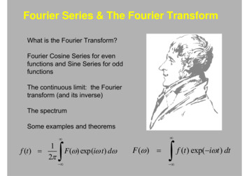
Anharmonic waves are sums of sinusoids.Consider the sum of two sine waves (i.e., harmonic waves) ofdifferent frequencies:The resulting wave is periodic, but not harmonic.Essentially all waves are anharmonic.

FourierdecomposingfunctionsHere, we write asquare wave asa sum of sine waves.

Any function can be written as thesum of an even and an odd functionLet f(x) be any function.E(-x) E(x)E(x)E ( x ) [ f ( x ) f ( x )] / 2O(x)O(-x) -O(x)O ( x ) [ f ( x ) f ( x )] / 2 f(x)f ( x) E ( x) O ( x)

Fourier Cosine SeriesBecause cos(mt) is an even function (for all m), we can write an evenfunction, f(t), as:f(t) F π1mcos(mt)m 0where the set {Fm; m 0, 1, } is a set of coefficients that define theseries.And where we’ll only worry about the function f(t) over the interval(–π,π).

The Kronecker delta functionδ m,n 1 if m n 0 if m n

Finding the coefficients, Fm, in a Fourier Cosine SeriesFourier Cosine Series:1f (t ) π Fm cos( mt )m 0To find Fm, multiply each side by cos(m’t), where m’ is another integer, and integrate:π πBut:πSo: π 1f (t) cos(m' t) dt πm 0π f (t ) cos(m ' t ) dt π1π π π if m m ' π δ m ,m ' 0 if m m 'cos( mt ) cos( m ' t ) dt πFm cos(mt) cos(m' t) dt Fm π δ m,m 'Å only the m’ m term contributesm 0πDropping the ‘ from the m:Fm πf (t ) cos(mt ) dtÅ yields thecoefficients forany f(t)!

Fourier Sine SeriesBecause sin(mt) is an odd function (for all m), we can writeany odd function, f(t), as: f (t) 1πFm′ sin(mt)m 0where the set {F’m; m 0, 1, } is a set of coefficients that definethe series.where we’ll only worry about the function f(t) over the interval (–π,π).

Finding the coefficients, F’m, in a Fourier Sine Series Fourier Sine Series:f (t) 1πFm′ sin(mt)m 0To find Fm, multiply each side by sin(m’t), where m’ is another integer, and integrate:π f (t ) sin(m ' t ) dt πF ′ sin(mt ) sin( m ' t ) dt π1mm 0 πBut: ππ π if m m 'sin(mt ) sin(m ' t ) dt π δ m,m ' 0 if m m ' π So:π f (t ) sin(m ' t ) dt π F′ π δ π1mm,m 'Å only the m’ m term contributesm 0πDropping the ‘ from the m:Fm′ πf (t ) sin(mt ) dt Å yields the coefficientsfor any f(t)!

Fourier SeriesSo if f(t) is a general function, neither even nor odd, it can bewritten:f (t ) 1 πm 01 πFm cos(mt ) m 0even componentFm′ sin(mt )odd componentwhereFm f (t) cos(mt) dtandFm′ f (t) sin(mt) dt

We can plot the coefficients of a Fourier Series1Fm vs. m.5051025152030mWe really need two such plots, one for the cosine series and anotherfor the sine series.

Discrete Fourier Series vs.Continuous Fourier TransformFm vs. mLet the integerm become areal numberand let thecoefficients,Fm, become afunction F(m).F(m)mAgain, we really need two such plots, one for the cosine series andanother for the sine series.

The Fourier TransformConsider the Fourier coefficients. Let’s define a function F(m) thatincorporates both cosine and sine series coefficients, with the sineseries distinguished by making it the imaginary component:F(m) Fm – i F’m f (t ) cos(mt ) dt i f (t ) sin(mt ) dtLet’s now allow f(t) to range from – to , so we’ll have to integratefrom – to , and let’s redefine m to be the “frequency,” which we’llnow call ω: F (ω) f (t) exp( iω t) dtThe FourierTransform F(ω) is called the Fourier Transform of f(t). It contains equivalentinformation to that in f(t). We say that f(t) lives in the time domain,and F(ω) lives in the frequency domain. F(ω) is just another way oflooking at a function or wave.

The Inverse Fourier TransformThe Fourier Transform takes us from f(t) to F(ω).How about going back?Recall our formula for the Fourier Series of f(t) :f (t ) 1π Fm cos( mt ) m 01π Fm' sin( mt )m 0Now transform the sums to integrals from – to , and again replaceFm with F(ω). Remembering the fact that we introduced a factor of i(and including a factor of 2 that just crops up), we have:1f (t ) 2π F (ω) exp(iωt ) dωInverseFourierTransform

Fourier Transform NotationThere are several ways to denote the Fourier transform of afunction.If the function is labeled by a lower-case letter, such as f,we can write:f(t) F(ω)If the function is labeled by an upper-case letter, such as E, we canwrite:E (t ) Y {E (t )}or: Sometimes, this symbol isused instead of the arrow:E (t ) E% (ω )

The SpectrumWe define the spectrum, S(ω), of a wave E(t) to be:S (ω ) Y {E (t )}2This is the measure of the frequencies present in a light wave.

Example: the Fourier Transform of arectangle function: rect(t)1/ 21F (ω ) exp( iω t ) dt [exp( iω t )]1/ 1/2 2 iω 1/ 21[exp( iω / 2) exp(iω /2)] iω1 exp(iω / 2) exp( iω /2) 2i(ω /2)sin(ω /2) sinc(ω /2)(ω /2) F {rect(t )} sinc(ω/2)F(ω)ImaginaryComponent 0ω

Example: the Fourier Transform of adecaying exponential: exp(-at) (t 0) F (ω ) exp( at ) exp( iωt )dt0 00 exp( at iωt )dt exp( [a iω ]t )dt 1 1 exp( [a iω ]t ) 0 [exp( ) exp(0)]a iωa iω 1[0 1] a iω1 a iω 1F (ω ) iω iaA complex Lorentzian!

Example: the Fourier Transform of aGaussian, exp(-at2), is itself! F {exp( at 2 )} 2exp( at) exp( iωt ) dt exp( ω / 4a )2The details are a HW problem!exp( ω / 4a )exp( at )22 0t0ω

Fourier Transform Symmetry PropertiesExpanding the Fourier transform of a function, f(t): F (ω) [Re{ f (t )} i Im{ f (t )}] [cos(ωt ) i sin(ωt )] dt Expanding more, noting that: O(t) dt 0if O(t) is an odd function F (ω ) i 0 if Re{f(t)} is odd Re{ f (t )} cos(ω t ) dt 0 if Im{f(t)} is odd Im{ f (t )} cos(ω t ) dt i Even functions of ω 0 if Im{f(t)} is even Im{ f (t )} sin(ω t) dt 0 if Re{f(t)} is even Re{ f (t )} sin(ω t) dt Odd functions of ω Re{F(ω)} Im{F(ω)}

The Dirac delta functionUnlike the Kronecker delta-function, which is a function of twointegers, the Dirac delta function is a function of a real variable, t. if t 0δ (t ) 0 if t 0δ(t)t

The Dirac delta function if t 0δ (t ) 0 if t 0It’s best to think of the delta function as the limit of a series ofpeaked continuous functions.fm(t) m exp[-(mt)2]/ πδ(t)f3(t)f2(t)f1(t)t

Dirac δ function Propertiesδ(t) δ (t ) dt 1t δ (t a ) f (t ) dt δ (t a ) f ( a ) dt exp( iω t ) dt 2π δ (ω ) exp[ i (ω ω ′)t ] dt 2π δ (ω ω ′ )f (a)

The Fourier Transform of δ(t) is 1. δ (t ) exp( iωt ) dt exp( iω [0]) 1 δ(t)1ωt And the Fourier Transform of 1 is 2πδ(ω): 1 exp( iωt ) dt 2π δ (ω ) 2πδ(ω)1tω

The Fourier transform of exp(iω0 t) F{exp(iω0 t )} exp(iω0 t ) exp( i ω t ) dt exp( i [ω ω0 ] t ) dt 2π δ (ω ω0 ) exp(iω0t)Im0Re0Y {exp(iω0t)}tt0ω0ωThe function exp(iω0t) is the essential component of Fourier analysis.It is a pure frequency.

The Fourier transform of cos(ω0 t) F{cos(ω0t )}1 21 2 cos(ω0t ) exp( i ω t ) dt [ exp(i ω0 t ) exp( i ω0 t )] exp( i ω t ) dt exp( i [ω ω0 ] t ) dt 12 exp( i [ω ω0 ] t ) dt π δ (ω ω0 ) π δ (ω ω0 )F {cos(ω0t )}cos(ω0t)0t ω00 ω0ω

The Modulation Theorem:The Fourier Transform of E(t) cos(ω0 t)F{E (t ) cos(ω0t )}1 2 1 2 E (t ) cos(ω0t ) exp( i ω t ) dt E (t ) exp(i ω0t ) exp( i ω0t ) exp( i ω t ) dt E (t ) exp( i [ω ω ] t ) dt0 12 E (t ) exp( i [ω ω ]t ) dt0 1 %F { E (t ) cos(ω0t )} E (ω ω0 ) 2Example:E (t ) cos(ω0t )F1 %E (ω ω0 )2{E (t ) cos(ω0t )}E(t) exp(-t2)t-ω00ω0ω

Scale TheoremF { f ( at )} F (ω /a ) / aThe Fourier transformof a scaled function, f(at): Proof: F { f (at )} f (at ) exp( iω t ) dt Assuming a 0, change variables: u at F { f (at )} f (u ) exp( iω [ u /a ]) du / a f (u) exp( i [ω /a] u) du / a F (ω /a) / aIf a 0, the limits flip when we change variables, introducing aminus sign, hence the absolute value.

F(ω)f(t)The ScaleTheoremin actionThe shorterthe pulse,the broaderthe spectrum!This is the essenceof the thpulseLongpulse

The FourierTransform of asum of twofunctionsF(ω)f(t)G(ω)g(t)F {a f (t) bg(t)} aF { f (t)} bF {g(t)}tf(t) g(t)Also, constants factor out.ωttωF(ω) G(ω)ω

Shift TheoremThe Fourier transform of a shifted function, f (t a ) :F{ f (t a)} exp( iω a) F (ω )Proof : F{ f ( t a )} f (t a ) exp( iωt )dt Change variables : u t a f (u ) exp( iω[u a ])du exp( iω a ) f (u ) exp( iωu )du exp( iω a ) F (ω )

Fourier Transform with respect to spaceIf f(x) is a function of position,F (k ) f ( x) exp( ikx) dxxY {f(x)} F(k)We refer to k as the spatial frequency.kEverything we’ve said about Fourier transforms between the t and ωdomains also applies to the x and k domains.

The 2D Fourier TransformY If(2){f(x,y)} f(x,y) F(kx,ky)f(x,y) exp[-i(kxx kyy)] dx dyf(x,y) fx(x) fy(y),then the 2D FT splits into two 1D FT's.But this doesn’t always happen.xYy(2){f(x,y)}

The Pulse WidthΔtThere are many definitions of the"width" or “length” of a wave or pulse.tThe effective width is the width of a rectangle whose height andarea are the same as those of the pulse.f(0)Effective width Area / height: Δteff1 f (t ) dt f (0) Δteff(Abs value isunnecessaryfor intensity.)Advantage: It’s easy to understand.Disadvantages: The Abs value is inconvenient.We must integrate to .0t

The rms pulse widthΔtThe root-mean-squared width orrms width: 2 t f (t ) dt f (t ) dt Δtrmst1/ 2The rms width is the “second-order moment.”Advantages: Integrals are often easy to do analytically.Disadvantages: It weights wings even more heavily,so it’s difficult to use for experiments, which can't scan to )

The aximumis the distance between thehalf-maximum points.Advantages: Experimentally easy.Disadvantages: It ignores satellitepulses with heights 49.99% of thepeak!tΔtFWHMtAlso: we can define these widths in terms of f(t) or of its intensity, f(t) 2.Define spectral widths (Δω) similarly in the frequency domain (t ω).

The Uncertainty PrincipleThe Uncertainty Principle says that the product of a function's widthsin the time domain (Δt) and the frequency domain (Δω) has a minimum.Define the widthsassuming f(t) andF(ω) peak at 0: 1f (t ) dtΔt f (0) 1F (ω ) dωΔω F (0) 11F (0)f (t ) dt f (t ) exp( i[0] t ) dt Δt f (0) f (0) f (0) 112π f (0)(ω)ω(ω)exp(ωωΔω Fd Fi[0])d F (0) F (0) F (0)Combining results:f (0) F (0)Δω Δt 2πF (0) f (0)(Different definitions of the widths and theFourier Transform yield different constants.)or:Δ ω Δ t 2πΔν Δt 1

The Uncertainty PrincipleFor the rms width, Δω Δt ½There’s an uncertainty relation for x and k: Δk Δx ½

physics of heat and developed the Fourier series and transform to model heat-flow problems. Anharmonic waves are sums of sinusoids. Consider the sum of two sine waves (i.e., harmonic waves) of different frequencies: The resulting wave is periodic