WIXLIB

111.4. WHY STUDY THE SHO? 0/0/ /0/00/0/ /0/00/0/ /0/0 0/0/0/0/ &%&% %&%&&%&% %&%&%&&% %&%& 43 34434321 34321443214321 32143214314221 13241221 12 0/0/ &%&%.-.- -.-.-.- -.-.-.- -.-.&%&%%&&% # # # # # # # # # # # # 43434321 # #31422121 .-.-.-, , , ,, , , ,, , , , # # # #"!"! !"!""!!" !"!""!"! !"!"43214321.-.-"!"!, , , , , , *)*) )*)**))* )*)**)*) )*)*"!!""!"!('(' '('(('(' '('(('(' '('(*)*)*))**)*)('('('('('('Figure 1.5:It is very useful to remember that hcos(ω0 t φ)i 0. This can be easilyverified by noting that the values sin(ω0 t φ) are bound between 1 and 1. We use this to calculate the average kinetic and potential energiesboth of which have the same values1hU i hT i mω02 A2 .4(1.14)The average kinetic and potential energies, and the total energy are allvery conveniently expressed in the complex representation as11E/2 hU i hT i mṽṽ kx̃x̃ 44(1.15)where denotes the conjugate of a complex number.Problem 3: The mean displacementof a SHO hxi is zero. The root meanq2square (rms.) displacement hx i is useful in quantifying the amplitude ofoscillation. Verify that the rms. displacement isSolution:qx̃x̃ /21.4qhx2 (t)i qA2 hcos2 (ω0t φ)i qqx̃x̃ /2.A2 /2 qÃeiω Ã e iωt /2 Why study the SHO?What happens to a system when it is disturbed from stable equilibrium? Thisquestion that arises in a large variety of situations. For example, the atoms inmany solids (eg. NACl, diamond and steel) are arranged in a periodic crystalas shown in Figure 1.5. The periodic crystal is known to be an equilibriumconfiguration of the atoms. The atoms are continuously disturbed from theirequilibrium positions (shown in Figure 1.5) as a consequence of random thermal motions and external forces which may happen to act on the solid. Thestudy of oscillations in the atoms disturbed from their equilibrium position isvery interesting. In fact the oscillations of the different atoms are coupled, and

12CHAPTER 1. OSCILLATIONSV(x) xV(x)2V(x) exp(x 2/2) 12V(x) x x3xFigure 1.6:this gives rise to collective vibrations of the whole crystal which can explainproperties like the specific heat capacity of the solid. We shall come back tothis later, right now the crucial point is that each atom behaves like a SHO ifwe assume that all the other atoms remain fixed. This is generic to all systemswhich are slightly disturbed from stable equilibrium.We now show that any potential V (x) is well represented by a SHO potential in the neighbourhood of points of stable equilibrium. The origin of x ischosen so that the point of stable equilibrium is located at x 0. For smallvalues of x it is possible to approximate the function V (x) using a Taylor seriesdV (x)V (x) V (x)x 0 dx!1x 2x 0d2 V (x)dx2!x2 .(1.16)x 0where the higher powers of x are assumed to be negligibly small. We know thatat the points of stable equilibrium the force vanishes ie. F dV (x)/dx 0and V (x) has a minimak d2 V (x)dx2! 0.(1.17)x 0This tells us that the potential is approximately1V (x) V (x)x 0 kx22(1.18)which is a SHO potential. Figure 1.6 shows two different potentials which arewell approximated by the same SHO potential in the neighbourhood of thepoint of stable equilibrium. The oscillation frequency is exactly the same forparticles slightly disturbed from equilibrium in these three different potentials.The study of SHO is important because it occurs in a large variety ofsituations where the system is slightly disturbed from equilibrium. We discussa few simple situations.

131.4. WHY STUDY THE SHO?765765765 765765765 765765765 765765765 757575756765 765 765 75giqlCθLmFigure 1.7: (a) and (b)Simple pendulumThe simple possible shown in Figure 1.7(a) is possibly familiar to all of us.A mass m is suspended by a rigid rod of length l, the rod is assumed to bemassless. The gravitations potential energy of the mass isV (θ) mgl[1 cos θ] .(1.19)For small θ we may approximate cos θ 1 θ 2 /2 whereby the potential is1V (θ) mglθ 22(1.20)which is the SHO potential. Here dV (θ)/dθ gives the torque not the force.The pendulum’s equation of motion isI θ̈ mglθ(1.21)where I ml2 is the moment of inertia. This can be written asgθ̈ θ 0l(1.22)which allows us to determine the angular frequencyω0 rgl(1.23)LC OscillatorThe LC circuit shown in Figure 1.7(b) is an example of an electrical circuitwhich is a SHO. It is governed by the equationLI Q 0C(1.24)

14CHAPTER 1. OSCILLATIONSwhere L refers to the inductance, C capacitance, I current and Q charge. Thiscan be written as1Q̈ Q 0(1.25)LCwhich allows us to identifys1(1.26)ω0 LCas the angular frequency.Problems1. An empty tin can floating vertically in water is disturbed so that itexecutes vertical oscillations. The can weighs 100 gm, and its height andbase diameter are 20 and 10 cm respectively. [a.] Determine the periodof the oscillations. [b.] How much water need one pour into the can tomake the time period 1s?2. A SHO with ω0 2 s 1 has initial displacement and velocity 0.1 m and2.0 ms 1 respectively. [a.] At what distance from the equilibrium position does it come to rest? [b.] What are the rms. displacement andrms. velocity? What is the displacement at t π/4 s?3. A SHO with ω0 3 s 1 has initial displacement and velocity 0.2 m and2 ms 1 respectively. [a.] Expressing this as x̃(t) Ãeiω0 t , determineà a ib from the initial conditions. [b.] Using à Aeiφ , what are theamplitude A and phase φ for this oscillator? [c.] What are the initialposition and velocity if the phase is increased by π/3?224. A particle of mass m 0.3 kg in the potential V (x) 2ex /L J (L 0.1 m) is found to behave like a SHO for small displacements from equilibrium. Determine the period of this SHO.5. Calculate the time average hx4 i for the SHO x A cos ωt.

Chapter 2The Damped Oscillator.Damping usually comes into play whenever we consider motion. We study theeffect of damping on the spring-mass system. The damping force is assumedto be proportional to the velocity, acting to oppose the motion. The totalforce acting on the mass isF kx cẋ(2.1)where in addition to the restoring force kx due to the spring we also havethe damping force cẋ. The equation of motion for the damped spring masssystem ismẍ kx cẋ .(2.2)Recasting this in terms of more convenient coefficients, we haveẍ 2β ẋ ω02 x 0(2.3)This is a second order homogeneous equation with constant coefficients. Bothω0 and β have dimensions (time) 1 . Here 1/ω0 is the time-scale of the oscillations that would occur if there was no damping, and 1/β is the time-scalerequired for damping to bring any motion to rest. It is clear that the natureof the motion depends on which time-scale 1/ω0 or 1/β is larger.We proceed to solve equation (2.4) by taking a trial solutionx(t) Aeαt .(2.4)Putting the trial solution into equation (2.4) gives us the quadratic equationα2 2βα ω 2 0This has two solutionsandα1 β α2 β qβ 2 ω2qβ 2 ω2(2.5)(2.6)(2.7)The nature of the solution depends critically on the value of the dampingcoefficient β, and the behaviour is quite different depending on whether β ω0 ,β ω0 or β ω0 .15

16CHAPTER 2. THE DAMPED OSCILLATOR.1x(t) e t cos(20 t)0.5x0 0.5 1012t345Figure 2.1:2.1Underdamped OscillationsWe first consider the situation where β ω0 which is referred to as underdamped. Definingqω ω02 β 2(2.8)the two roots which are both complex have valuesα1 β iω and α2 β iω(2.9)The resulting solution is a superposition of the two rootsx(t) e βt [A1 eiωt A2 e iωt ](2.10)where A1 and A2 are constants which have to be determined from the initialconditions. The term [A1 eiωt A1 eiωt ] is a superposition of sin and cos whichcan be written asx(t) Ae βt cos(ωt φ)(2.11)This can also be expressed in the complex notation asx̃(t) Ãe(iω β)t(2.12)where à Aeiφ is the complex amplitude which has both the amplitudeand phase information. Figure 2.1 shows the underdamped motion x(t) e t cos(2πt).In all cases damping reduces the frequency of the oscillations ie. ω ω0 .The main effect of damping is that it causes the amplitude of the oscillationsto decay exponentially with time. It is often useful to quantify the decay inthe amplitude during the time period of a single oscillation T 2π/ω. Thisis quantified by the logarithmic decrement which is defined as"#2πβx(t) λ lnx(t T )ω(2.13)

172.2. OVER-DAMPED 522.533.54tFigure 2.2:Problem 1.: An under-damped oscillator with x̃(t) Ãe(iω β)t has initialdisplacement and velocity x0 and v0 respectively. Calculate à and obtain x(t)in terms of the initial conditions.Solution: à x0 i(v0 βx0 )/ω and x(t) e βt [x0 cos ωt ((v0 βx0 )/ω) sin ωt].2.2Over-damped Oscillations.This refers to the situation whereβ ω0The two roots areandα1 β qα2 β q(2.14)β 2 ω02 γ1(2.15)β 2 ω02 γ2(2.16)where both γ1 , γ2 0 and γ2 γ1 . The two roots give rise to exponentiallydecaying solutions, one which decays faster than the otherx(t) A1 e γ1 t A2 e γ2 t .(2.17)The constants A1 and A2 are determined by the initial conditions. For initialposition x0 and velocity v0 we havev0 γ2 x0 γ1 t v0 γ1 x0 γ2 te e(2.18)x(t) γ2 γ 1γ2 γ 1The overdamped oscillator does not oscillate. Figure 2.2 shows a typicalsituation.In the situation where β ω0qβ2 ω02 vuuβ t1 and we have γ1 ω02 /2β and γ2 2β."1 ω02ω02 β1 β22 β2#(2.19)

18CHAPTER 2. THE DAMPED 2.533.54tFigure 2.3:2.3Critical Damping.This corresponds to a situation where β ω0 and the two roots are equal.The governing equation is second order and there still are two independentsolutions. The general solution isx(t) e βt [A1 A2 t](2.20)x(t) x0 e βt [1 βt](2.21)The solutionis for an oscillator starting from rest at x0 whilex(t) v0 e βt t(2.22)is for a particle starting from x 0 with speed v0 . Figure 2.3 shows the lattersituation.2.4SummaryThere are two physical effects at play in a damped oscillator. The first isthe damping which tries to bring any motion to a stop. This operates on atime-scale Td 1/β. The restoring force exerted by the spring tries to makethe system oscillate and this operates on a time-scale T0 1/ω0 . We haveoverdamped oscillations if the damping operates on a shorter time-scale compared to the oscillations ie. Td T0 which completely destroys the oscillatorybehaviour.Figure 2.4 shows the behaviour of a damped oscillator under different combinations of damping and restoring force. The plot is for ω0 1, it can be usedfor any other value of the natural frequency by suitably scaling the values of β.It shows how the decay rate for the two exponentially decaying overdampedsolutions varies with β. Note that for one of the modes the decay rate tendsto zero as β is increased. This indicates that for very large damping a particlemay get stuck at a position away from equilibrium.

192.4. 100.511.522.53βFigure 2.4:Problems1. Obtain solution (2.20) for critical damping as a limiting case (β ω0 )of overdamped solution (2.18).2. Find out the conditions for the initial displacement x(0) and the initialvelocity ẋ(0) at t 0 such that an overdamped oscillator crosses themean position once in a finite time.3. An under-damped oscillator has a time period of 2s and the amplitudeof oscillation goes down by 10% in one oscillation. [a.] What is thelogarithmic decrement λ of the oscillator? [b.] Determine the dampingcoefficient β. [c.] What would be the time period of this oscillator ifthere was no damping? [d.] What should be β if the time period is tobe increased to 4s? ([a.] 1.05 10 1 [b.] 2.7 10 2 s 1 [c.]2s [d.] 2.72s 14. Two identical under-damped oscillators have damping coefficient andangular frequency β and ω respectively. At t 0 one oscillator is atrest with displacement a0 while the other has velocity v0 and is at theequilibrium position. What is the phase difference between these twooscillators. (π/2 tan 1 (β/ω))5. A door-shutter has a spring which, in the absence of damping, shuts thedoor in 0.5s. The problem is that the door bangs with a speed 1m/sat the instant that it shuts. A damper with damping coefficient β isintroduced to ensure that the door shuts gradually. What are the timerequired for the door to shut and the velocity of the door at the instantit shuts if β 0.5π and β 0.9π? Note that the spring is unstretchedwhen the door is shut. (0.57s, 4.67 10 1 m/s; 1.14s, 8.96 10 2 m/s)6. An LCR circuit has an inductance L 1 mH, a capacitance C 0.1 µFand resistance R 250Ω in series. The capacitor has a voltage 10 V atthe instant t 0 when the circuit is completed. What is the voltageacross the capacitor after 10µs and 20µs? (7.64 V, 4.84 V )

20CHAPTER 2. THE DAMPED OSCILLATOR.7. A highly damped oscillator with ω0 2 s 1 and β 104 s 1 is givenan initial displacement of 2 m and left at rest. What is the oscillator’sposition at t 2 s and t 104 s? (2.00 m, 2.70 10 1 m)8. A critically damped oscillator with β 2 s 1 is initially at x 0 withvelocity 6 m s 1 . What is the furthest distance the oscillator moves fromthe origin? (1.10 m)9. A critically damped oscillator is initially at x 0 with velocity v0 . Whatis the ratio of the maximum kinetic energy to the maximum potentialenergy of this oscillator? (e2 )10. An overdamped oscillator is initially at x x0 . What initial velocity, v0 ,should be the given to the oscillator that it reaches the mean position(x 0) in the minimum possible time.11. We have shown that the general solution, x(t), with two constants candescribe the motion of damped oscillator satisfying given initial conditions. Show that there does not exist any other solution satisfying thesame initial conditions.

Chapter 3Oscillator with external forcing.In this chapter we consider an oscillator under the influence of an externalsinusoidal force F cos(ωt ψ). Why this particular form of the force? Thisis because nearly any arbitrary time varying force F (t) can be decomposedinto the sum of sinusoidal forces of different frequenciesF (t) XFn cos(ωn t ψn )(3.1)n 1,.Here Fn and ψn are respectively the amplitude and phase of the differentfrequency components. Such an expansion is called a Fourier series. The behaviour of the oscillator under the influence of the force F (t) can be determinedby separately solvingmx n kxn Fn cos(ωn t ψn )(3.2)for a force with a single frequency and then superposing the solutionsx(t) Xxn (t) .(3.3)nWe shall henceforth restrict our attention to equation (3.2) which has asinusoidal force of a single frequency and drop the subscript n from xn andFn . It is convenient to switch over to the complex notation ω02 x̃ f eiωtx̃(3.4)where f F eiψ /m.3.1Complementary function and particular integralThe solution is a sum of two partsx̃(t) Ãeiω0 t B̃eiωt .21(3.5)

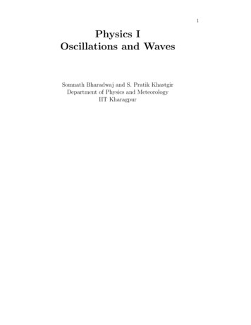
22 φCHAPTER 3. OSCILLATOR WITH EXTERNAL FORCING.PHASEπ010AMPLITUDE8f ω 10 x Resonance64f/ ω 020022f/ ω0.51ω1.52Figure 3.1: Amplitue and phase as a function of forcing frequncyThe first term Ãeiω0 t , called the complementary function, is a solution to equation (3.4) without the external force. This oscillates at the natural frequencyof the oscillator ω0 . This part of the solution is exactly the same as when thereis no external force. This has been discussed extensively earlier, and we shallignore this term in the rest of this chapter.The second term B̃eiωt , called the particular integral, is the extra ingredientin the solution due to the external force. This oscillates at the frequency of theexternal force ω. The amplitude B̃ is determined from equation (3.4) whichgives[ ω 2 ω02 ]B̃ f (3.6)whereby we have the solutionx̃(t) f eiωt .22ω0 ω(3.7)The amplitude and phase of the oscillation both depend on the forcingfrequency ω. The amplitude is x̃ ω02f. ω2 (3.8)and the phase of the oscillations relative to the applied force is φ 0 forω ω0 and φ π for ω ω0 .Note: One cannot decide here whether the oscillations lag or lead thedriving force, i.e. whether φ π or φ π as both of them are consistentwith ω ω0 case (e iπ 1). The zero resistance limit, β 0, of the dampedforced oscillations (which is to be done in the next section) would settle it forφ π for ω ω0 . So in this case there is an abrupt change of π radiansin the phase as the forcing frequency, ω, crosses the natural frequency, ω0 .The amplitude and phase are shown in Figure 3.1. The first point to noteis that the amplitude increases dramatically as ω ω0 and the amplitudeblows up at ω ω0 . This is the phenomenon of resonance. The response of

233.2. EFFECT OF DAMPINGthe oscillator is maximum when the frequency of the external force matchesthe natural frequency of the oscillator. In a real situation the amplitude isregulated by the presence of damping which ensures that it does not blow upto infinity at ω ω0 .We next consider the low frequency ω ω0 behaviourx̃(t) f iωt F i(ωt φ)e e,ω02k(3.9)The oscillations have an amplitude F/k and are in phase with the externalforce.This behaviour is easy to understand if we consider ω 0 which is aconstant force. We know that the spring gets e

The book \Oscillations and waves" is an account of one semester course, PHYSICS-I, given by the authors for the last three years at IIT, Kharagpur. The book is targeted at the rst year undergraduate science and engineering students. Starting with oscillations in