Transcription
ewNeret h rss tein a pt a chonC n ewAn Introduction toANSYS Fluent 2020 Vector Based ImageJohn E. Matsson, Ph.D., P.E.SDCP U B L I C AT I O N SBetter Textbooks. Lower Prices.www.SDCpublications.com
Visit the following websites to learn more about this book:Powered by TCPDF (www.tcpdf.org)
CHAPTER 2. FLAT PLATE BOUNDARY LAYERCHAPTER 2. FLAT PLATE BOUNDARY LAYERA. Objectives Creating Geometry in ANSYS Workbench for ANSYS Fluent Flow SimulationSetting up ANSYS Fluent Simulation for Laminar Steady 2D Planar FlowSetting up MeshSelecting Boundary ConditionsRunning CalculationsUsing Plots to Visualize Resulting Flow FieldCompare with Theoretical Solution using Mathematica CodeB. Problem DescriptionIn this chapter, we will use ANSYS Fluent to study the two-dimensional laminar flow on a horizontalflat plate. The size of the plate is considered as being infinite in the spanwise direction and thereforethe flow is 2D instead of 3D. The inlet velocity for the 1 m long plate is 5 m/s and we will be usingair as the fluid for laminar simulations. We will determine the velocity profiles and plot the profiles.We will start by creating the geometry needed for the simulation.C. Launching ANSYS Workbench and Selecting Fluent1. Start by launching ANSYS Workbench. Double click on Fluid Flow (Fluent) that is located underAnalysis Systems in Toolbox.Figure 2.1 Selecting Fluid Flow19
CHAPTER 2. FLAT PLATE BOUNDARY LAYERD. Launching ANSYS DesignModeler2. Select Geometry under Project Schematic in ANSYS Workbench. Right-click on Geometry andselect Properties. Select 2D Analysis Type under Advanced Geometry Options in Properties ofSchematic A2: Geometry. Right-click on Geometry in Project Schematic and select to launchNew DesignModeler Geometry. Select Units Millimeter as the length unit from the menu inDesignModeler.Figure 2.2a) Selecting Geometry and 2D Analysis TypeFigure 2.2b) Launching DesignModelerFigure 2.2c) Selecting the length unit20
CHAPTER 2. FLAT PLATE BOUNDARY LAYER3. Next, we will be creating the geometry in DesignModeler. Select XYPlane from the Tree Outlineon the left-hand side in DesignModeler. Select Look at Sketchin the Tree Outline and select the Line sketch tool. Click on the Sketching tabDraw a horizontal line 1,000 mm long from the origin to the right. Make sure you have a P at theorigin when you start drawing the line. Also, make sure you have an H along the line so that it ishorizontal and a C at the end of the line.Select Dimensions within the Sketching options. Click on the line and enter a length of 1,000mm. Draw a vertical line upward 100 mm long starting at the end point of the first horizontal line.Make sure you have a P when starting the line and a V indicating a vertical line. Continue with ahorizontal line 100 mm long to the left from the origin followed by another vertical line 100 mmlong.The next line will be horizontal with a length 100 mm starting at the endpoint of the formervertical line and directed to the right. Finally, close the rectangle with a 1,000 mm long horizontalline starting 100 mm above the origin and directed to the right.Figure 2.3a) Selection of XYPlaneFigure 2.3b) Selection of Line tool21
CHAPTER 2. FLAT PLATE BOUNDARY LAYERFigure 2.3c) Rectangle with dimensionsFigure 2.3d) Dimensions in Details View4. Click on the Modeling tab under Sketching Toolboxes. Select Concept Surfaces from Sketchesin the menu. Control select the six edges of the rectangle as Base Objects and select Apply inDetails View. Click on Generate in the toolbar. The rectangle turns gray. Right clickin the graphics window and select Zoom to Fit and close DesignModeler.Figure 2.4a) Selecting Surfaces from SketchesFigure 2.4b) Applying Base Objects22
CHAPTER 2. FLAT PLATE BOUNDARY LAYERFigure 2.4c) Completed rectangle in DesignModelerE. Launching ANSYS Meshing5. We are now going to double click on Mesh under Project Schematic in ANSYS Workbench toopen the Meshing window. Select Mesh in the Outline of the Meshing window. Right click andselect Generate Mesh. A coarse mesh is created. Select Unit Systems Metric (mm, kg, N )from the bottom of the graphics window.Figure 2.5a) Launching meshFigure 2.5b) Generating meshFigure 2.5c) Coarse meshFigure 2.5d) Selection of units in graphics window23
CHAPTER 2. FLAT PLATE BOUNDARY LAYERSelect Mesh Controls Face Meshing from the menu. Click on the yellow region next toGeometry under Scope in Details of Face Meshing. Select the rectangle in the graphics window.Click on the Apply button for Geometry in Details of “Face Meshing”. Select Mesh Controls Sizing from the menu and select Edgeabove the graphics window.Figure 2.5e) Selection of face meshing Figure 2.5f) SizingSelect the upper longer horizontal edge of the rectangle, control select the lower horizontal edgesand the vertical edges for a total of 5 edges. Click on Apply for the Geometry in “Details of EdgeSizing”. Under Definition in “Details of Edge Sizing”, select Element Size as Type, 1.0 mm forElement Size, and Hard as Behavior. Select the second Bias Typeand enter 12.0 asthe Bias Factor.Figure 2.5g) Details of edge sizing for three of the horizontal edges and the vertical edgesRepeat the selection of Mesh Controls Sizing from the menu once again but this time selectthe upper horizontal edge to the left of the origin. Enter the same Element Size, Behavior, andBias Factor but the first Bias Type. Click on Home Generate Mesh in the menuand select Mesh in the Outline. The finished mesh is shown in the graphics window.24
CHAPTER 2. FLAT PLATE BOUNDARY LAYERFigure 2.5h) Details of edge sizing for the remaining horizontal edgeFigure 2.5i) Details of finished meshWhy did we create a biased mesh? The reason for using a biased mesh isthat we need a finer mesh close to the wall where we have velocity gradientsin the flow. We also included a finer mesh where the boundary layer starts todevelop on the flat plate.We are now going to rename the edges for the rectangle. Select the left edge of the rectangle,right click and select Create Named Selection. Enter inlet as the name and click on the OKbutton.Repeat this step for the right vertical edge of the rectangle and enter the name outlet. Create anamed selection for the lower longer horizontal right edge and call it wall. Finally, control-selectthe remaining three horizontal edges and name them ideal wall. An ideal wall is an adiabatic andfrictionless wall.25
CHAPTER 2. FLAT PLATE BOUNDARY LAYERFigure 2.5j) Named selectionsSelect File Export Mesh FLUENT Input File Export from the menu. Select Save astype: FLUENT Input Files (*.msh). Enter “boundary-layer-mesh” as file name and click on theSave button. Select File Save Project from the menu. Name the project “Flat Plate BoundaryLayer”. Close the ANSYS Meshing window. Right click on Mesh in Project Schematic and selectUpdate.F. Launching ANSYS Fluent6. We are now going to double click on Setup under Project Schematic in ANSYS Workbench toopen Fluent. Launch the Dimension 2D and Double Precision solver of Fluent. Check the DoublePrecision. Set the number of Solver Processes equal to the number of computer cores. To checkthe number of physical cores, press the Ctrl Shift Esc keys simultaneously to open the TaskManager. Go to the Performance tab and select CPU from the left column. You'll see the numberof physical cores on the bottom-right side. Click on Show More Options. Write down the locationof the working directory as you will use this information later. Click on the Start button to launchANSYS Fluent.Why do we use double precision? Double precision will give moreaccurate calculations than single precision.Figure 2.6a) Launching Setup26
CHAPTER 2. FLAT PLATE BOUNDARY LAYERFigure 2.6b) TaskmanagerFigure 2.6c) Fluent Launcher27
CHAPTER 2. FLAT PLATE BOUNDARY LAYERFigure 2.6d) Example of console printout for four cores7. Check the scale of the mesh by selecting the Scale button under Mesh in General on the TaskPage. Make sure that the Domain Extent is correct and close the Scale Mesh window.Figure 2.7a) Scale CheckFigure 2.7b) Scale Mesh8. Double click on Models and Viscous (SST k-omega). Select Laminar as Viscous Model. ClickOk to close the window. Double click on Boundary Conditions under Setup in the Outline View.Double click on inlet under Zone on the Task Page. Choose Components as VelocitySpecification Method and set the X-Velocity (m/s) to 5. Click on the OK button to close thewindow. Double click on ideal wall under Zones. Check Specified Shear as Shear Condition andkeep zero values for specified shear stress since an ideal wall is frictionless. Click OK to close thewindow.Why did we select Laminar as Viscous Model? For the chosen free streamvelocity 5 m/s the Reynolds number is less than 500,000 along the plate andthe flow is therefore laminar. Turbulent from along a flat plate occurs atReynolds numbers above 500,000.28
CHAPTER 2. FLAT PLATE BOUNDARY LAYERFigure 2.8a) Viscous modelFigure 2.8b) Boundary Conditions for inletFigure 2.8c) Inlet velocity29
CHAPTER 2. FLAT PLATE BOUNDARY LAYERFigure 2.8d) Specified shear for ideal wall9. Double click on Methods under Solution in the Outline View. Select Standard for Pressure andFirst Order Upwind for Momentum. Double click on Reference Values under Setup in theOutline View. Select Compute from inlet on the Task Page.Figure 2.9a) Solution Methods Task PageWhy do we use First Order Upwind method for Spatial Discretization ofMomentum? The First Order Upwind method is generally less accurate but convergesbetter than the Second Order Upwind method. It is common practice to start with theFirst Order Upwind method at the beginning of calculations and continue with theSecond Order Upwind method.30
CHAPTER 2. FLAT PLATE BOUNDARY LAYERFigure 2.9b) Reference values10. Double click on Initialization under Solution in the Outline View, select Standard Initialization,select Compute from inlet, and click on the Initialize button.Figure 2.10 Solution Initialization31
CHAPTER 2. FLAT PLATE BOUNDARY LAYER11. Double click on Monitors under Solution in the Outline View. Double click on Residual underMonitors and enter 1e-9 as Absolute Criteria for all Residuals. Click on the OK button to closethe window.Figure 2.11a) Residual monitorsFigure 2.11b) Residual Monitors settingsWhy did we set the Absolute Criteria to 1e-9? Generally, the lower the absolutecriteria, the longer time the calculation will take and give a more exact solution. Wesee in Figure 2.12b) that the x-velocity and y-velocity equations have lower residualsthan the continuity equation. The slopes of the residual curves for all three equationsare about the same with a sharp downward trend.32
CHAPTER 2. FLAT PLATE BOUNDARY LAYER12. Double click on Run Calculation under Solution and enter 5000 for Number of Iterations. Clickon the Calculate button.Figure 2.12a) Running the calculationsFigure 2.12b) Scaled Residuals33
CHAPTER 2. FLAT PLATE BOUNDARY LAYERG. Post-Processing13. Select the Results tab in the menu and select Create Line/Rake under Surface. Enter 0.2 for x0(m), 0.2 for x1 (m), 0 for y0 (m), and 0.02 m for y1 (m). Enter x 0.2m for the New Surface Nameand click on Create. Repeat this step three more times and create vertical lines at x 0.4m (length0.04 m), x 0.6m (length 0.06 m), and x 0.8m (length 0.08 m). Close the window.Figure 2.13a) Selecting Line/Rake from the Post-processing menuFigure 2.13b) Line/Rake Surfaces at x 0.2 m and x 0.4m14. Double click on Plots and XY Plot under Results in the Outline View. Uncheck Position on XAxis under Options and check Position on Y Axis. Set Plot Direction for X to 0 and 1 for Y.Select Velocity and X Velocity as X Axis Function. Select the four surfaces x 0.2m, x 0.4m,x 0.6m, and x 0.8m.34
CHAPTER 2. FLAT PLATE BOUNDARY LAYERFigure 2.14a) XY Plot setupFigure 2.14b) Settings for Solution XY Plot35
CHAPTER 2. FLAT PLATE BOUNDARY LAYER15. Click on the Axes button in the Solution XY Plot window. Select the X Axis, uncheck AutoRange under Options, enter 6 for Maximum Range, select general Type under Number Formatand set Precision to 0. Click on the Apply button. Select the Y Axis, uncheck the Auto Range,enter 0.01 for Maximum Range, select general Type under Number Format, and click on theApply button. Close the Axes window.Figure 2.15a) Settings for X AxesFigure 2.15b) Settings for Y Axes36
CHAPTER 2. FLAT PLATE BOUNDARY LAYER16. Click on the Curves button in the Solution XY Plot window. Select the first pattern under LineStyle for Curve # 0. Select no Symbol for Marker Style and click on the Apply button.Next select Curve # 1, select the next available Pattern for Line Style, no Symbol for MarkerStyle, and click on the Apply button. Continue this pattern of selection with the next two curves #2 and # 3. Close the Curves – Solution XY Plot window. Click on the Save/Plot button in theSolution XY Plot window and close this window.Figure 2.16a) Settings for curve # 0Figure 2.16b) Velocity profiles for a laminar boundary layer on a flat plate37
CHAPTER 2. FLAT PLATE BOUNDARY LAYERSelect the User Defined tab in the menu and Custom. Select a specific Operand Field Functionsfrom the drop-down menu by selecting Mesh and Y-Coordinate. Click on Select and enter thedefinition as shown in Figure 2.16e). You need to select Mesh and X-Coordinate to completethe definition of the field function. Enter eta as New Function Name, click on Define and closethe window.Repeat this step to create another custom field function. This time, we select Velocity and XVelocity as Field Functions and click on Select. Complete the Definition as shown in Figure2.16f) and enter u-divided-by-freestream-velocity as New Function Name, click on Define andclose the window.Figure 2.16c) Custom Field FunctionsFigure 2.16d) Operand Field FunctionFigure 2.16e) Custom field function for self-similar coordinateWhy did we create a self-similar coordinate? It turns out that by using a self-similarcoordinate, the velocity profiles at different streamwise positions will collapse on oneself-similar velocity profile that is independent of the streamwise location.38
CHAPTER 2. FLAT PLATE BOUNDARY LAYERFigure 2.16f) Custom field function for non-dimensional velocity17. Double click on Plots and XY Plot under Results in the Outline View. Set X to 0 and Y to 1 asPlot Direction. Uncheck Position on X Axis and Position on Y Axis under Options. Select CustomField Functions and eta for Y Axis Function and select Custom Field Functions and u-divided-byfreestream-velocity for X Axis Function.Place the file “blasius.dat” in your working directory. This file can be downloaded fromsdcpublications.com. See Figure 2.19 for the Mathematica code that can be used to generate thetheoretical Blasius velocity profile for laminar boundary layer flow over a flat plate. As anexample, in this case the working directory is 𝐶𝐶:\Users\jmatsson. Click on Load File. SelectFiles of type: All Files (*) and select the file “blasius.dat” from your working directory. Selectthe four surfaces x 0.2m, x 0.4m, x 0.6m, x 0.8m and the loaded file Theory.Figure 2.17a) Solution XY Plot for self-similar velocity profiles39
CHAPTER 2. FLAT PLATE BOUNDARY LAYERClick on the Axes button. Select Y Axis in Axes-Solution XY Plot window and uncheck AutoRange. Set the Minimum Range to 0 and Maximum Range to 10. Set the Type to float andPrecision to 0 under Number Format. Enter the Label as eta and click on Apply.Select X Axis in Axes-Solution XY Plot window and enter the Label to u/U. Check the box forAuto Range. Set the Type to float and Precision to 1 under Number Format. Click on Apply andclose the window.Click on the Curves button in the Solution XY Plot window. Select the first pattern under LineStyle for Curve # 0. Select no Symbol for Marker Style and click on the Apply button.Next select Curve # 1, select the next available Pattern for Line Style, no Symbol for MarkerStyle, and click on the Apply button. Continue this pattern of selection with the next two curves #2 and # 3. Close the Curves – Solution XY Plot window. Click on the Save/Plot button in theSolution XY Plot window and close this window.Figure 2.17b) Axes – Solution XY Plot window settings for Y Axis40
CHAPTER 2. FLAT PLATE BOUNDARY LAYERFigure 2.17c) Axes – Solution XY Plot window settings for X AxisFigure 2.17d) Self-similar velocity profiles for a laminar boundary layer on a flat plate41
CHAPTER 2. FLAT PLATE BOUNDARY LAYERSelect the User Defined tab in the menu and Custom. Select a specific Operand Field Functionsfrom the drop-down menu by selecting Mesh and X-Coordinate. Click on Select and enter thedefinition as shown in Figure 2.17e). Enter re-x as New Function Name, click on Define andClose the window.Figure 2.17e) Custom field function for Reynolds number18. Double click on Plots and XY Plot under Results in the Outline View. Set X to 0 and Y to 1under Plot Direction. Uncheck Position on X Axis and Position on Y Axis under Options. SelectWall Fluxes and Skin Friction Coefficient for Y Axis Function and select Custom Field Functionsand re-x for X Axis Function.Place the file “Theoretical Skin Friction Coefficient” in your working directory. Click on LoadFile. Select Files of type: All Files (*) and select the file “Theoretical Skin Friction Coefficient”.Select wall under Surfaces and the loaded file Skin Friction under File Data. Click on the Axesbutton.Figure 2.18a) Solution XY Plot for skin friction coefficient42
CHAPTER 2. FLAT PLATE BOUNDARY LAYERCheck the X Axis, check the box for Log under Options, enter Re-x as Label, uncheck AutoRange under Options, set Minimum to 100 and Maximum to 1000000. Set Type to float andPrecision to 0 under Number Format and click on Apply.Check the Y Axis, check the box for Log under Options, enter Cf-x as Label, uncheck AutoRange, set Minimum to 0.001 and Maximum to 0.1, set Type to float, Precision to 3 and click onApply. Close the window. Click on Save/Plot in the Solution XY Plot window.Click on the Curves button in the Solution XY Plot window. Select the first pattern under LineStyle for Curve # 0. Select no Symbol for Marker Style and click on the Apply button.Next select Curve # 1, select the next available Pattern for Line Style, no Symbol for MarkerStyle, and click on the Apply button. Close the Curves – Solution XY Plot window. Click on theSave/Plot button in the Solution XY Plot window and close this window.Figure 2.18b) Axes – Solution XY Plot window settings for X AxisFigure 2.18c) Axes – Solution XY Plot window settings for Y Axis43
CHAPTER 2. FLAT PLATE BOUNDARY LAYERFigure 2.18d) Comparison between ANSYS Fluent and theoretical skin friction coefficient(dashed line) for laminar boundary layer flow on a flat plateH. Theory19. In this chapter we have compared ANSYS Fluent velocity profiles with the theoretical Blasiusvelocity profile for laminar flow on a flat plate. We transformed the wall normal coordinate to asimilarity coordinate for comparison of profiles at different streamwise locations. The similaritycoordinate is defined by𝑈𝑈𝜈𝜈𝜈𝜈𝜂𝜂 𝑦𝑦 where y (m) is the wall normal coordinate, U (m/s) is the free stream velocity, x (m) is thedistance from the streamwise origin of the wall and 𝜈𝜈 (m2/s) is the kinematic viscosity of thefluid.(2.1)We also used the non-dimensional streamwise velocity u/U where u is the dimensional velocityprofile. u/U was plotted versus 𝜂𝜂 for ANSYS Fluent velocity profiles in comparison with theBlasius theoretical profile and they all collapsed on the same curve as per definition of selfsimilarity. The Blasius boundary layer equation is given by44
CHAPTER 2. FLAT PLATE BOUNDARY LAYER1𝑓𝑓(𝜂𝜂)𝑓𝑓 ′′ (𝜂𝜂)2𝑓𝑓 ′′′ (𝜂𝜂) 0(2.2)with the following boundary conditions𝑓𝑓(0) 𝑓𝑓 ′ (0) 0, 𝑓𝑓 ′ ( ) 0(2.3)The Reynolds number for the flow on a flat plat is defined ��𝑅𝑅𝑅𝑥𝑥 The boundary layer thickness 𝛿𝛿 is defined as the distance from the wall to the location where thevelocity in the boundary layer has reached 99% of the free stream value. For a laminar boundarylayer we have the following theoretical expression for the variation of the boundary layerthickness with streamwise distance x and Reynolds number 𝑅𝑅𝑅𝑅𝑥𝑥 .𝛿𝛿 𝑅𝑅𝑅𝑅𝑥𝑥The corresponding expression for the boundary layer thickness in a turbulent boundary layer isgiven by𝛿𝛿 0.16𝑥𝑥(2.6)1/7𝑅𝑅𝑅𝑅𝑥𝑥The local skin friction coefficient is defined as the local wall shear stress divided by dynamicpressure.𝐶𝐶𝑓𝑓,𝑥𝑥 1𝜏𝜏𝑤𝑤(2.7)𝜌𝜌𝑈𝑈 22The theoretical local friction coefficient for laminar flow is determined by𝐶𝐶𝑓𝑓,𝑥𝑥 0.664𝐶𝐶𝑓𝑓,𝑥𝑥 0.027 𝑅𝑅𝑅𝑅𝑥𝑥𝑅𝑅𝑅𝑅𝑥𝑥 5 105(2.8)5 105 𝑅𝑅𝑅𝑅𝑥𝑥 107(2.9)and for turbulent flow we have the following relation1/7𝑅𝑅𝑅𝑅𝑥𝑥45
CHAPTER 2. FLAT PLATE BOUNDARY LAYERFigure 2.19 Mathematica code for theoretical Blasius laminar boundary layerI. References1.2.3.4.Çengel, Y. A., and Cimbala J.M., Fluid Mechanics Fundamentals and Applications, 1st Edition,McGraw-Hill, 2006.Richards, S., Cimbala, J.M., Martin, K., ANSYS Workbench Tutorial – Boundary Layer on a FlatPlate, Penn State University, 18 May 2010 Revision.Schlichting, H., and Gersten, K., Boundary Layer Theory, 8th Revised and EnlargedEdition, Springer, 2001.White, F. M., Fluid Mechanics, 4th Edition, McGraw-Hill, 1999.J. Exercises2.1 Use the results from the ANSYS Fluent simulation in this chapter to determine the boundarylayer thickness at the streamwise positions as shown in the table below. Fill in the missinginformation in the table. 𝑈𝑈𝛿𝛿 is the velocity of the boundary layer at the distance from the wallequal to the boundary layer thickness and U is the free stream velocity.x (m)0.2𝛿𝛿 (𝑚𝑚𝑚𝑚)Fluent𝛿𝛿 (𝑚𝑚𝑚𝑚)TheoryPercentDifference𝑈𝑈 4.00001460.6.00001460.8.0000146𝑅𝑅𝑅𝑅 𝑥𝑥Table 2.1 Comparison between Fluent and theory for boundary layer thickness46
CHAPTER 2. FLAT PLATE BOUNDARY LAYER2.2 Change the element size to 2 mm for the mesh and compare the results in XY Plots of theskin friction coefficient versus Reynolds number with the element size 1 mm that was used inthis chapter. Compare your results with theory.2.3 Change the free stream velocity to 3 m/s and create an XY Plot including velocity profiles atx 0.1, 0.3, 0.5, 0.7 and 0.9 m. Create another XY Plot with self-similar velocity profiles forthis lower free stream velocity and create an XY Plot for the skin friction coefficient versusReynolds number.2.4 Use the results from the ANSYS Fluent simulation in Exercise 2.3 to determine the boundarylayer thickness at the streamwise positions as shown in the table below. Fill in the missinginformation in the table. 𝑈𝑈𝛿𝛿 is the velocity of the boundary layer at the distance from the wallequal to the boundary layer thickness and U is the free stream velocity.x (m)0.1𝛿𝛿 (𝑚𝑚𝑚𝑚)Fluent𝛿𝛿 (𝑚𝑚𝑚𝑚)TheoryPercentDifference𝑈𝑈 𝑅𝑅 𝑥𝑥Table 2.2 Comparison between Fluent and theory for boundary layer thickness47
CHAPTER 2. FLAT PLATE BOUNDARY LAYERK. Notes48
C. Launching ANSYS Workbench and Selecting Fluent . 1. Start by launching ANSYS Workbench. Double click on Fluid Flow (Fluent) that is located under Analysis Systems in Toolbox. Figure 2.1 Selecting Fluid Flow . CHAPTER 2. FLAT PLATE BOUNDARY LAY