Transcription
ANSYS Fluent Tutorial Part 1This tutorial introduces you to the ANSYS workbench and Fluent environments. Upon completing thistutorial you will understand: ANSYS workbench environmento Create a new project, create geometry, mesh the domain, identify and name boundaryconditions, grid adaptationFlow simulation in Fluento Export mesh to Fluent, apply boundary conditions, iterate toward the solution, examine theflow fields, obtain numerical results, examine and validate the resultsProject 1 description:Simulate fluid flow through a rectangular channel shown below.2 cmWallVelocityOutflowWall10 cmFigure 1.1Consider air flowing through a rectangular channel of 2cm height and 10cm length. Assume that the channelhas an infinite width. Inlet air velocity is 0.1 / at the inlet and outlet is at the atmospheric pressure.1
1 ANSYYS Workbbench1.1 Open Workbench1.2.3.4.Opeen the Start MenuMTyppe Workbenchh into the seaarchSeleect the icon foor Workbencch 17.1Alteernately, you can find it in the ANSYS 17.1 folder of thestarrt menu1.2 Creaate a Fluid FlowF(Fluentt) Project1. Undder the Toolbox tab (leftt menu), draag the FLUENNTmoodule over too the Workspace (white space) ordouuble‐click.2. Youu will see youur new Projeect appear. Name itProoject 1 Laminnar Flow Coaarse Mesh. ThisT willdiffferentiate thhe project filee from somee of the otheerflueent simulatioons you will be creating.3. Savve the projecct in your U:// drive.3Project BoxxToolboox12FigureF1.22Figuree 1.1
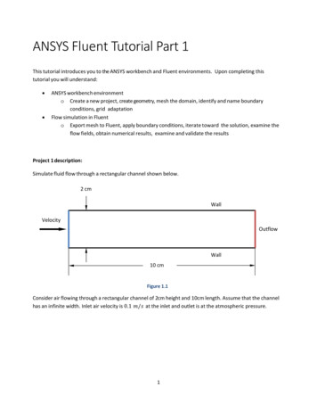
1.3 Set upu Workbennch Informaation1. On the top menuu, click View2. Seleect Files. A meenu will pop up at the botttom. This ca n tell you where the files aare stored. TTherewill be a bunch createdcas you progress annd it may be i mportant to note the locaation.3. On the top menuu again, click View, and select Propertiees. This timee, a menu will appear on thherighht side of the screen. The Properties menumwill channge as you select differentt tabs on yourrprojject.12PPropertiess Menu3Files MenuFigureF1.33
1.4 Set AnalysisAtype1. Witthin your Prooject box, sinngle‐click Geeometry. Your Propertiees menu will change.2. Undder Advanceed Geometryy Options, seet Analysis TType to 2D.12Fiigure 1.41.5 Neww Geometry1. In thet Project Box,B right‐click Geometryy.2. Seleect New Dessign Modeleer Geometryy 3. ANSSYS Design ModelerM(DMM) will thenopeen.Note thhat you can also Import Geometry ifyou maade the geommetry in a CAAD program.Just savve the CAD filef as a univversal formatt,such ass .STPFigure 1.54
2 ANSYYS Design Modelerr2.1 Creaating a New Sketch1. In the Tree Outliine (left menuu), click XYPlaane2. In the Top Menuu, click the Neew Sketch icoon. Sketch 1 wwill appear inn your Tree OOutline underXYPPlane3. On the Coordinaate System in the bottom‐right corner, click the Z‐aaxis to snap yyour view to 22D inthe XY plane. Yoou can also familiarize yourself with thee zooming andd panning funnctions.4. To beginbdrawingg the geomettry, select thee Sketching taab at the botttom of the Trree Outline. NNotethatt the Sketchinng Toolboxess menu will reeplace your TTree Outline.2. New Sketch1Tree Ouutline43FigureF2.15
2.2 Drawwing the Geeometry1. In the Sketching Toolbox, undder Draw, clicck Rectangle. Your cursorr will become a pencil.2. Create the rectangle of any siize anywhere in Quadrant 1 of your draawing canvas. We will connstrainthe location and size next.Drawwing ToolsEditing ToolsFigureF2.22.3 Consstraining Geeometry to the Axis1. In the Sketching Toolbox, select the Consttraints dropd own.ect Coincidennce. This will set a rule forr an edge to ccoincide with another.2. Sele3. Click the edge off the rectangle you want too constrain a nd then selecct the axis youu want to lock it to.Thee edges of thee rectangle wiill change color if they are fully constrained.4. Do thist for both edges of the rectangle, soo that its loweer left corner is at the origiin (0, 0).FigureF2.36
2.4 Dimeensioning thhe Geometry1. In the Sketching Toolbox, seleect the Dimennsions dropdoown2. Seleect General. You can also use Horizonttal or Vertica l for their resspective lines.3. Seleect the edge ofo the rectanggle you want to dimensionn. Click abovee or next to that edge to pplacethe dimension laabel.e a dimensionn, it will showw up in the Deetails View mmenu. You cann edit these vvalues4. When you created it will adjustt the size of thhe rectangle.and5. Create a dimension for the hoorizontal and vertical liness of the rectanngle and set ttheir values tood 2 0.02 , respectively.1 0.1 andFigureF2.47
2.5 Creeating a Surrface1.2.3.4.Cllick back to thhe Modeling Tab at the boottom of the SSketching Tooolbox.OnO the top meenu, open thee Concept droopdown and sselect Surfacee from Sketchhes.Seelect your skeetch and thenn click Apply ini the Detailss View (bottoom left menu)).Cllick the Geneerate button in the top menu. Your parrt will fill grayy when the suurface isgeenerated.5. Yoou are now done with creaating your geometry. Clickk Save and close Design MModeler.4213Figure 2.58
3 Meshing3.1 Oppen Meshingg1.2.3.4.5.GoG back into ANSYS Worrkbench.NoteNthat youu should seee a checkmarrk next to Geeometry in yyour Projectt Box.Saave the Projject.Inn the Projectt Box, right‐click Mesh anda select Eddit The Mesh Editor will opeen and your GeometryGshould autommatically load.Figure 3.19
3.2 Sett up Meshinng1. WithW the Meshh Editor openn, orient your view, if neceessary, with thhe coordinatee system anddZooom to Fit (button in the TopT Menu with a Cube insside a Magnifyying Glass). YYou can alsofaamiliarize youurself with thee zooming and panning fu nctions.2. Inn the Outline menu (left side), expand outo the Geommetry tree (plus sign) and cclick Surface Body3. Thhe Details Meenu (bottom left) will channge to properrties of the Suurface Body4. Under the Deffinition tab, change the Thhickness to.5. Under the Matterial tab, chaange the Fluid/Solid to Fluuid.Figure 3.210
3.3 Sett Mesh Resoolution1.2.3.4.Inn the Outline menu, click thet Mesh tab.Thhe Details meenu will change to propertties of the Meesh.Seet Min Size, MaxM Face Sizee, and Max Teet Size all toThhis will set yoour grid size too 1 mm spacing.Figure 3.311.
3.4 Sett Mesh to QuadrilateraQals1. Faamiliarize youurself with the types of sellection tools. There is Verrtex Selectionn, Edge Selection,Faace Selectionn, and Body Selection.2. Use the Face SelectionStooll to select thee face of the ggeometry3. OnceOit is seleccted (the facee turns green)), right‐click tthe geometryy and Insert MMapped FaceMeshingM4. A Face Meshinng will appearr in your Outlline menu. OOnce it is seleccted, the Details menu willshhow its propeerties.5. Inn the Details Menu,Mmake sure Methodd is set to Quaadrilaterals.6. Inn the top mennu, click Geneerate Mesh. If you click thhe Mesh icon in the Outlinne menu again,yoour mesh shoould appear overoyour geometry.162435Figure 3.412
3.5 Boundary Labbeling1.2.3.4.Inn the Top Menu, use the edgeeselectionn tool to selecct the left edge of your geeometryRight‐click the left edge andd select Creatte Named Se lectionNameNthis edgge inlet.wall top, wall bottom, anRepeat the proocess for the other edges, naming the wnd outflow,espectively.re5. Thhis naming prrocess helps FluentFdetermmine Boundarry Conditionss.6. Click File, Savee Project, andd return to ANNSYS. If you wwant to creatte a backup file of the Messh,ou can select File, Export, and change thet file type t o .msh. If forr some reasonn, youryoWorkbenchWPrroject becomees corrupted, you can resuume from thiss point by impporting the .mmshfile to a new Project. Note that you will not be able tto edit your .mmsh file, so innspect that it isorrect before exporting.coFigure 3.513
4 Flueent4.1 Upddating Projeect1. Back in Workbeench, you mayy notice a Ligghtning Bolt nnext to the MMesh in your PProject Box. TThiseans that youur Mesh has notn been updaated yet.me2. To update the Mesh,Mright‐cclick Mesh andd select Updaate. Once it is done, a greeen checkmarrkshoould appear.Fiigure 4.14.2 Starrting Fluentt1. To open Fluent,, double‐clickk Setup in the Project Box. A dialog will pop up withh settings. Selectthee following opptions and click OK.Fiigure 4.214
4.3 Flueent Layout1. Fluuent is segmeented into sevveral menus.a. Top Ribbbon – Adjustting propertieesb. Tree – EachEstep of settingsup thee simulationc. Task Paage – The setuup of variablees and properrties in each sstep of the Trreed. Main WindowW– Vieww the domainn, simulation progress, or resultse. Consolee – The commmand line shoowing progresss or errors.2. Opperating Fluennt will mainly consist of running down tthe Tree and editing variables in eachresspective Taskk Page.abdceFiigure 4.315
4.4 Setuup – GeneraalNote: Recoommended seelections for ProjectP1 are in Bold and UUnderlined1. Meeshygeometrry and mesh sshould autommatically display. If it doessn’t,a. Once Fluent opens, yourn manually dissplay componnents by clickking Display inn the Task Paage.you canb. If you need to scale the geometryy (e.g. you maade the geommetry in inchees and you waantthe soluution in SI uniits), you can alsoa do it heree.c. You may also Check the mesh forr errors and qquality here.2. Solvera. Typeowsi. Pressure‐Based for low‐sspeed incomppressible to high‐speed compressible floed reserved forf flows withh strong interddependence between dennsity,ii. Density‐Baseenergy, mommentum, or species.nb. Velocityy Formulationi. Absolute is wherewmajoriity of the dommain is non‐rootationalii. Relative mayy be useful in cases wheree the domain rotatesc. Timees for a steady‐state (deveeloped) solutioni. Steady solveolution is a fu nction in timeii. Transient is used if the sod. 2D spaccei. Planar is youur standard 2D space in Caartesian coorddinateshe domain aroound an axis (e.g. cylindriccal coordinatees)ii. Axisymmetric revolves thiii. Axisymmetric swirl revolvves the domaain around ann axis with somme tangentialvelocity3. Gravity can include buoyancy effects for flowsfor graviitational settlling in particlee tracking.Fiigure 4.416
4.5 Setuup – ModelsDescriptionns:1. Energy trackingg is used for heathtransfer solutionssandd things that aare a functionn of temperatturea density, reelative humidity)(e.g. diffusion, airh you solvee/simplify thee Navier‐Stokkes equations. For Laminar2. Visscous Model determines howflow, simply chooose the Lamminar model. For Turbulennt flow, you have several ooptions thatsThee most common is k‐epsiloon because off its simplicityy.approximate a solution.u would simulate a speciess (e.g. relativee humidity) mmixing/diffusing3. Species trackingg is when young within the fluid.4. Disscrete Phase is used for paarticle trackinFiigure 4.517
4.6 Setuup – MateriialsIf you wantt to change environmental conditions, such as the wworking fluid (e.g. air, wateer, helium) orrmaterial suurface roughnness (affects skins friction), you can do itt in this tabDefault prooperties are fine.fFiigure 4.6Note that CellC Zone Connditions will beb skipped over (defaults aare fine).18
4.7 Setuup – Boundary ConditionsThis is wheere we’ll definne the boundary conditionns for the sim ulation. Notee that the edgges you labeledduring messhing corresppond to the booundaries fouund in fluent. Select a zonne and click Eddit 1. Inlet – Set your Velocity Maggnitude to 0.1 m/sutflow – default weighting of 1. If you havehmultiplee outflows, yoou can scale tthe proportion of2. Outhee mass flow that exits eachh outflow (e.gg. 0.2 outfloww 1, 0.8 outfloow 2)3. Waall – Both deffault stationary wall with non slip. For o ther cases, yoou may want a moving waall.Fiigure 4.719
4.8 Soluution – Soluution Methoods1. Schhemea. SIMPLEE – (Semi‐Implicit Method forf Pressure‐ Linked Equattions) Defaultt, robust.b. SIMPLEC – (SIMPLE‐CConsistent) AllowsAfaster cconvergence for simple prroblems (e.g.,,laminarr flows with non physical moodels employyed)c. PISO – (Pressure‐Imp(plicit with Spllitting of Ope rators) For unnsteady flow problems ormesh withw high skewwness2. GradientGauss Cell Baased – Default method, so lution may haave false diffuusion/smearinga. Green‐Gb. Green‐GGauss Node BasedB– Minimmizes false difffusion, recommmended forr tri/tet meshhc. Least Sqquares Cell Baased – For poolyhedral messhes, same acccuracy, propperties as nodeessure3. Prea. Standarrd – The defaault scheme. ReducedRaccuuracy for flowws with large ssurface‐normmalpressurre gradients nearnboundaries (but shou ld not be useed when steepp pressurechangess are presentt in the flow – PRESTO! schheme should be used insteead)b. PRESTOO! – For highlyy swirling flowws, steep presssure gradiennts, or curvedd domainsc. Linear – When otherr options resuult in converggence difficultties or unphysical behaviord. Second‐Order – Use for compresssible flowse. Body Foorce Weighted – When forrces are largee e.g. high Ra convection, sswirling flowss4. Moomentumd very diffusivvea. First Orrder Upwind – Easiest convvergence, onlly first order aaccurate, andi.e. dissipates large gradientsgandd can suppres s small/sharpp featuresndnd – 2 order accuracy, esssential whenn flow is not aaligned withb. Second Order Upwinmesh grid direction e.g.e during tri/tet meshFiigure 4.820
4.9 Soluution – Monnitors1. Select Residualss and click Eddit 2. Unnder Residual Values, checck the box thaat says Normaalize. This scales the last iiteration ofResiduals by thee maximum ResidualsRand can be used as a better gauge for convvergence.3. Unnder Convergeence Criterion, select Nonne. The Conv ergence Criteerion tells Fluent when theesollution has connverged to a value that yoou determine to be accuratte enough annd stopscallculating the solutionsearlyy. By turning this feature ooff, Fluent wiill continue caalculating theesollution until it reaches the numbernof iteerations you sset.Fiigure 4.921
4.10 Soluution – Soluution InitializationSelect yourr initializationn technique, thet boundaryy to initialize wwith, and theen click Initialize1. Staandard Initiallization – Thiss sets all mesh cells to a si ngle starting value. Typicaally, you selectvallues that are the closest too what you thhink the final solution will look like to help the solutiionconverge fasterr. Compute frrom Inlet takkes inlet cond itions (from tthe boundaryy conditions taabyou set earlier) and applies itt to the whole mesh as a sstarting guesss. The calculaations then reefinethee flow to a coonverged steaady‐state soluution2. Hyybrid Initialization – Provides a quick approximation of the flow field by solvingg Laplace’sequation to estimate a flow field and presssure field.Figgure 4.1022
4.11 Soluution – Run Calculationn(sometimes Fluent crashees). File, Savee Project1. SAAVE YOUR WOORK BEFORE PROCEEDINGP2. Check Case to makemsure eveerything is goood to go (youur mesh, boundary conditions, etc.)a. Note: Since I selected First order upwind earlieer, my Fluentt recommendded using a higherorder MomentumMSoolver (secondd order upwinnd) for improvved accuracy. This may bee agood suuggestion, so I went back tot solution m ethods and cchanged it. It also suggesteedLeast Sqquares for Gradient. You canc make thaat change tooo.ou can alwayss stop the calculation earlyy. Sometimes I’ll3. Sett the Numberr of Iterations to 1000. Yostoop at around 200 and checck that the floows/magnituddes make somme sense befoore spending allthaat time calculating to find out I made a mistake settiing the bounddary conditioons.4. Clicck CalculateFiggure 4.1123
4.12 Calcculating SolutionOnce the programpcalcuulates, you’ll sees a plot of thet residuals (errors) for eeach of the eqquationparameters (in this casee, continuity, x‐velocity, y‐vvelocity).Note that mym solution convergedcafter approximaately 400 iteraations to the minimum error.Also note thattthe Console prints thee residuals corresponding tto each iterattion.Once you haveha solutioon calculated,, save your work again.Figgure 4.1224
ANSYS Fluent Tutorial Part 1 This tutorial introduces you to the ANSYS workbench and Fluent environments. Upon completing this tutorial you will understand: ANSYS workbench environment o Create a new project, create geometry, mesh the domai