Transcription
Lighting Market ImpactEvaluation StudyModelling Assumptions ReportPrepared for NSW Office of Environment and HeritageNovember 2017DRAFT REPORT - V0.3
Table of ContentsTable of Contents . 21 Introduction . 32 Approach . 43 Derivation of Required Parameters . 53.1 Duration of Period 1 (Downlights) . 53.2Duration of Period 1 (Fluorescent and HID) . 63.3Duration of Period 2 . 63.4Electrical Power . 73.5Operating Hours . 94 Data Issues and Uncertainties. 10References . 11Annex - Graphs . 12
1 IntroductionThe purpose of this report is to outline the assumptions, their justification, and the datasources and approach taken to market modelling that was carried out as part of a LightingMarket Impact Evaluation Study (LMIES).For the purpose of the modelling and the LMIES, lighting in NSW commercial buildings wassplit into the following 4 sectors: Residential: common areas of apartment buildings. Office. Non-office commercial: retail, education, health, accommodation, hospitality and leisure. Industrial: factories and warehouses.The above 4 sectors represent the most granular level that commercial lighting was able tobe dissected to, given the available market data. Note that road/outdoor lighting was notmodelled in detail, as ESS activity in this sector has been negligible.The key lighting upgrade types were modelled, and each was categorised by sector. Theupgrade types modelled are listed below, and these are predominantly upgrades to LEDtechnology (although some historical ESS upgrades to T5 and similar technologies did takeplace): Downlight upgrades in residential buildings (for common areas, which are covered by theESS commercial lighting formula). Downlight upgrades in offices. Downlight upgrades in non-office commercial buildings. Fluorescent upgrades in offices. Fluorescent upgrades in non-office commercial buildings. Fluorescent upgrades in industrial buildings. HID upgrades in industrial buildings. HID upgrades in non-office commercial buildings.Note that these are the key upgrades that have dominated the ESS. Small quantities ofother upgrade types have also taken place however, for example downlight replacements inindustrial premises, HIDs in offices, etc.
2 ApproachIn order to accurately estimate the lifetime energy savings from upgrading a light (either anentire luminaire or simply a lamp-only replacement) logic dictates that we need to consider3 different lights: The existing light which is replaced - the “incumbent”. This is typically a halogen,fluorescent or HID. The light that is installed by an ACP - the “ESS” light. This is typically an LED. The light that would have replaced the incumbent, in the absence of the ESS, eitherwhen the incumbent fails or more likely when a major renovation of the space isundertaken. We call this light the “counterfactual”. We cannot know what thecounterfactual would have been, so this needs to be estimated using modelling andforecasting. Counterfactual installations are likely to include both LEDs and oldtechnology (halogen, fluorescent, HID). Some building owners will fit LEDs when lightsfail or the space is renovated, and some will opt to stay with old technology. Thecounterfactual is the weighted average light that would have been installed (weighted byquantities of installations).Figure 1 below illustrates these three lights, on a time scale.Figure 1 - sequence of lights used to calculate energy savingsTime ------------------- IncumbentESSCounterfactual ------ period 1 -------- ------ period 2 -------- In order to calculate the total energy savings from the installation of the ESS light, we needto calculate (and sum together) energy savings over the two distinct periods illustrated inthe figure above: period 1 and period 2. To do this we need to calculate the followingparameters: The duration of periods 1 and 2 - refer sections 3.1, 3.2 and 3.3. The electrical power of the incumbent, ESS and counterfactual lights - refer section 3.4. The annual operating hours of the lights - refer section 3.5.The derivation of all the required parameters is discussed in the following sections.
3 Derivation of Required Parameters3.1 Duration of Period 1 (Downlights)Period 1 is the remaining life of the incumbent light - the length of time before it would havebeen replaced by the counterfactual (in the absence of the ESS). The assumption used isthat the incumbent light is half way through its life, when the ESS unit is installed and period1 commences. This assumption is intuitive - if you select a large quantity of lights at random,then on average they will be half way through their life.Note however that lights targeted for replacement by ACPs are of course not selected atrandom, and technologies such as halogen are rapidly receding from the market (referFigure 4 in Annex). Thus, halogen lights are likely to be more than half way through their life(e.g. remaining halogens are quite likely to be replaced by LED at the end of their life intuitively this means that any remaining halogens are relatively old).Thus, the assumption that the incumbent light is half way through its life will tend to overestimate energy savings (by over-estimating the duration of period 1). However, in theabsence of better data we have stayed with this 50% assumption.The other piece of information we need to calculate the duration of period 1 is the total lifeof the incumbent (which we then halve, i.e. based on the 50% assumption).For downlights (all sectors) one approach that can be taken is that halogen downlights canbe easily replaced with LED lamps, i.e. the entire fixture does not need to be replaced inorder to become LED. This is now common practice and effective and compatible LEDreplacement lamps are widely available.Using this “lamp-only” replacement approach, halogen lamps have typical rated lives of4,000-10,000 hours1 and using operating hours of 3,000-5,000 hours, then we have anestimated average lamp life of 0.8 - 3.3 years.An alternative approach is to assume that downlights are not likely to be replaced with LEDsuntil the space is renovated, at which time all the fixtures might be replaced with LEDs.Taking this approach, the total life of the incumbent would be much longer, i.e. in the orderof 10 years.Either of these approaches is possible, and on balance a hybrid of these approaches wasused - 4 years was used for the life of the incumbent (meaning that 2 years was used forperiod 1, for downlights). This approach is closer to the first method - the “lamp-only”method, however this was simply the subjective view of the author (i.e. that the lamp-onlyapproach to downlight replacement with LED was more common).1Taken from manufacturer catalogues (Sylvania Lighting Australasia, Philips Lighting, GE Lighting)
3.2 Duration of Period 1 (Fluorescent and HID)For fluorescent and HID lights, the assumption that the incumbent light is half way throughits life remains. However, LED lamp-only replacements for these kinds of lights are lesscommon than for halogen downlights. Thus, the approach taken was that total life of theincumbent is more likely to be the mean time between major renovations of the space inquestion. That is, lighting fixtures are typically replaced when the space is renovated.No data exists for the frequency of renovations. Thus, as part of stakeholder interviews forthe LMIES, stakeholders were asked for their opinion as to how often various building typesare typically renovated. On average, the responses were as follows: Office spaces: 10 years was widely touted, but noting that there is likely to be a verylarge range here - as low as 7 years for high quality office space, and much longer (e.g. 20years) for low quality office space. Non-office commercial spaces: 15 years. Industrial spaces: 20 years.These periods were then halved in order to calculate the duration of period 1. The resultsfor all upgrade types are shown in Table 1.Table 1 - values for duration of period 1Upgrade TypeLife of incumbent(years)Period 1 (years)Downlights - residential (common areas)4.02.0Downlights - offices4.02.0Downlights - non-office commercial buildings4.02.0Fluorescent - offices10.05.0Fluorescent - non-office commercial buildings15.07.5Fluorescent - industrial20.010.0HID - industrial20.010.0HID - non-office commercial buildings15.07.53.3 Duration of Period 2Referring to Figure 1, Period 2 can be expressed as the life of the ESS installation minus theduration of period 1.Logically, it can be argued that the life of the ESS installation is also equivalent to the meantime between renovations of the space in question, which is the approach used for Period 1.This also makes sense for LED downlights.However, in the case of industrial buildings, it did not seem prudent to assign a life of 20years to ESS installations. This would mean that installed LEDs would need to have lifetimes
of 100,000 hours (operating 5,000 hours p.a. x 20 years). Thus, for industrial applicationsthe life of the ESS installation was capped at 15 years.The resultant ESS installation lives, and durations for periods 1 and 2, are shown in Table 2.Table 2 - values for durations of periods 1 and 2Upgrade TypePeriod 1(years)ESS InstallationLife (years)Period 2(years)Downlights - residential (common areas)2.010.08.0Downlights - offices2.010.08.0Downlights - non-office commercial buildings2.010.08.0Fluorescent - offices5.010.05.0Fluorescent - non-office commercial buildings7.515.07.5Fluorescent - industrial10.015.05.0HID - industrial10.015.05.0HID - non-office commercial buildings7.515.07.53.4 Electrical PowerThe historical electrical power of the incumbent and ESS lights are known, i.e. from ACPlamp circuit power (LCP) data.The electrical power of the counterfactual is not known. To estimate this, we need toforecast the average quantities of LED and old-technology lights that we consider wouldhave been installed at the end of the incumbent’s life. We also need to estimate theelectrical power for each, then take a weighted average - the weighted averagecounterfactual.The power of the old-technology lights was assumed to remain static, as lightingmanufacturers are not investing in making these technologies more efficient. LEDs are,however, becoming more efficient and this is expected to continue. A future forecast of LEDefficacy was taken from a US study (US DoE 2016[A]) and from this the power of LEDs wasforecast.Extensive modelling was undertaken to forecast the following important metric: theestimated turnover rate, which is the percentage of retirements of incumbent lights thattransition to LED. The modeling was based primarily on ABS lamp import data (ABS 2017[B])(refer Figure 4) with trends extrapolated into the future. The Annex contains multiplegraphs for this metric, but Figure 2 below shows an example - the estimated turnover ratefor fluorescent fixtures in the non-office commercial sector.
Figure 2 - estimated turnover rate to LED, for fluorescent lights in non-office commercialsectorFrom the figure above we can see that, in 2016, an estimated 67% of remaining fluorescentfixtures are being replaced with LED fixtures, when they reach the end of their life (i.e. whenthe space is renovated). It is important to keep in mind that this percentage does pertain towhat happens during major renovation, when luminaires are typically replaced. In this case,two thirds of fluorescent lights are replaced with LED lights, when the space is upgraded.During interviews conducted for the LMIES, many (but not all) lighting suppliers stated thatthey now sell only LED luminaires. Whilst it is unlikely that 100% of new luminaire sales arenow LED, the 67% estimate above does appear conservative in light of the informationprovided by lighting suppliers, as does the assumption that the rate does not increasebeyond 80% in future.Graphs for all the upgrade types/sectors can be seen in the Annex.From this estimated turnover rate, and from forecasts of LED efficacy into the future, we canthen calculate the weighted average power of the counterfactual. Figure 3 below charts theresults of this modelling for the same example used above. It shows the following powervalues (for typical twin 4-foot fluorescent fixtures used in non-office commercial buildings): Incumbent - twin 36W lamp fixture with magnetic ballast, power 88W (from ESSformula). Counterfactual - the calculated weighted average of the incumbent technology and themarket average LED (weighted using the estimated turnover rate described above). i.e.some fixtures will be replaced like-for-like (fluorescent replacing fluorescent) and somewill upgrade to LED. Market average LED - the forecast power of the market average LED fixture.
ESS LED - the forecast power of the ESS LED installed (assumed to be 25% more efficientthan the market average LED, due to the inherent incentive for ESS lights to be moreefficient).Note that, throughout this report, these figures represent typical averages - there will ofcourse be installations that are larger and smaller than those shown in these graphs.Figure 3 - forecast power values for fluorescent lights in non-office commercial sectorFrom the figure above we can derive the following, for a typical ESS installation undertakenin 2016: The incumbent was an 88W fixture. It was replaced with an ESS LED of 42W. The counterfactual fixture would have been installed in 7.5 years time (2024) and it’spower would have been around 55W (the purple line in year 2024).Graphs for all the upgrade types/sectors can be seen in the annex.3.5 Operating HoursOperating hours, for the various sectors modelled, were taken from the ESS Rule.
4 Data Issues and UncertaintiesThe calculation approach outlined in previous sections is based on a number of assumptions,and also uses imperfect data. These issues are discussed in this section.Lighting is complex. In Australia, there are around half a billion lights installed (E3 2016a[C]).There are many different lighting technologies installed in many different types of buildingsand sectors, and we are in the middle of an unprecedented period of change in the availabletypes, efficiencies and costs of lights.To estimate the energy savings available from lighting upgrades, we need to examine thelighting stock - that is the quantities of the various types of lights actually installed inbuildings. However for various reasons very little data exists related to lighting stock.Counting of the stock of lights is occasionally undertaken by various organisations - forexample a modest residential stock count (E3 2016b[D]) was undertaken in 2016, with resultsbeing normalised using ABS household information. The challenges involved when countinglighting stock levels include: Lighting technologies are changing rapidly, meaning that counts become obsolete veryquickly. Lighting technologies can be can be difficult to identify in situ. Counting of a representative sample is a comprehensive and expensive exercise. Non-residential lighting stocks are considered more difficult to count, due to the widevariations in types of buildings, market sectors and lighting applications involved.Given these realities, we are forced to rely on desktop modelling for the commercial lightingsector, and this requires a large number of assumptions.In contrast to stock data, excellent data does exist for product sales - we have access to lampimport data2 (used a proxy for sales as no lamps are manufactured in Australia, and we don’thave access to sales data). These import data exist as a time series (refer Figure 4).However they do include limitations that they exists only at the national level - there is noavailable, state-level breakdown of commercial lighting market data, either for sales orstock.However, this import data series remains the best available time-series dataset for lighting.To take advantage of this rich data source, we need to convert sales data into stock, and forthis was done using a “stock-and-sales” model. The resultant model that was constructedfor this project is considered to be the best available lighting dataset ever developed forNew South Wales, although it does contain unavoidable uncertainty. From the model wealso derive the estimated turnover rates of lighting types, as these are critical inputs tocalculations of energy savings from lighting upgrades.ACP commercial lighting data was also collected from a number of ACPs, in order to estimatethe types and quantities of lighting being installed as part of the ESS. However this data onlycovered around 12% of the total ESS commercial lighting market. It was assumed that allESS commercial lighting activity occurred in the same proportions as this ACP data.2For conventional lamp types only - LEDs were not included in these data until January 2017.
To conclude , the key data issues and uncertainties can be summarised as follows: Predictions were made about the future efficacies of various LED lights, based on US DoE2016[A]. A number of assumptions were made about the durations of various lightinginstallations, based on interviews with stakeholders. The ACP commercial lighting installation data covered only around 12% of the ESScommercial lighting market. The ABS import lamp data, from which future trends regarding the uptake of LEDs wereextrapolated, exists only at the national level.References[A]US DoE 2016, Energy Savings Forecast of Solid-State Lighting in General IlluminationApplications, Prepared for the U.S. Department of Energy Solid-State Lighting Program,September 2016, Prepared by Navigant.[B]ABS 2017, Australian Bureau of Statistics, lamp import data, purchased from theAustralian Bureau of Statistics.[C]E3 2016a, Consultation Regulation Impact Statement - Lighting, Regulatory reformopportunities and improving energy efficiency outcomes, Energy Efficient EquipmentCommittee, November 2016.[D]E3 2016b, 2016 Residential Lighting Report, Results of a lighting audit of 180 Australianhomes, Energy Efficient Equipment Committee, June 2016.
Annex - GraphsABS DataExtensive modelling was undertaken to forecast the following important metric: theestimated turnover rate, which is the percentage of retirements of incumbent lights thattransition to LED. The modeling was based primarily on ABS lamp import data (ABS 2017[B])(refer Figure 4 below) with trends extrapolated into the future.Figure 4 - Import quantities of conventional lamp types, relative to 2010 quantities(source: ABS 2017[B])Graphs for Turnover RatesBelow are graphs of “turnover rates” for all upgrade types. This is the same type of graph asused as an example in Figure 2 in the main body of this report.
Graphs for Power ValuesBelow are graphs of average power values for all upgrade types. This is the same type ofgraph as used as an example in Figure 3 in the main body of this report.
1 Taken from manufacturer catalogues (Sylvania Lighting Australasia, Philips Lighting, GE Lighting) 3.2 Duration of Period 1 (Fluorescent and HID) For fluorescent and HID lights, th