WIXLIB

8.901 Course Notes4 How do we relate n and ρ? Sun is totally ionized, so both electrons and protonscontribute by number; but only protons contribute substantially to mass.:ρ mp n / 2 Then our requirement for classical physics means:m 2 me k T 3/ 2ρ por22h()3/ 2T classical, but only by a factor of 10. Not so far off!107 K Is the sun an ideal gas? If so, thermal energy dominates:kT e2 / a, soT e2 n1/3 / kT e2 (2 ρ / mp)1/3 / kT (15000 K) (ρ / 1g/cc)1/3This is satisfied throughout the entire sun: it’s valid to treat the Sun’s interior (and mostother stars) as an ideal gas.ρ (2800 g cm 3 )()

2. The Two-Body Problem and Kepler’s Laws210The Two-Body Problem and Kepler’s Laws

8.901 Course Notes5Lecture 2Space is Big.Last time we talked about mass scales; today we’ll talk about size scales: Bohr radius p2/2m hbar2 / (2 m a2) e2/a 5.3e-9 cm Rearth 6.3e8 cm (20000 / pi) km Rsun 7e10 cm 1 AU 1.5e13 cm 8 light-minutes 1 parsec 1 pc 3e18 cm 3.26 light years (note that l.y. are never used in astrophysics) Parsec is the fundamental unit of distance; it is the typical distance between stars (thoughthat’s just a coincidence). It is observationally defined:Earth’sorbit1 AU θd Over one year, the Earth’s displacement is 2 AU and an object at distance d changes apparentposition by 2θ, wheretan θ 1 AU / d, ord 1 AU / θ, ord / 1 pc 1 arcsec / θ Nearest star: 1.3 pcTo our galactic center: 8 kpc (kiloparsecs)To the nearest big galaxy: 620 kpc !! Cosmic Distance Ladder: Distance is a key concept in astrophysics – e.g. the revolution currently underway thanks toESA’s Gaia mission (measuring parallax for billions of objects with sub-milliarcsecprecision) “Distance ladder” refers to the bootstrapping of distance measurements, from nearby stars tothe furthest edges of the observable universe. Within solar system: light travel time. Radar, spacecraft communication, etc. Parallax: the first rung outside the Solar system. Measured by Gaia (2 nd data release) for 1billion stars across half of the Galaxy. A revolution is underway!

8.901 Course Notes6 Standard candles: if Luminosity L is known, then observed flux F gives distance:F L / 4 π d2 d (L / 4 π F)1/2Most important types: Cepheid variables - giant pulsating stars, period varies with absolute magnitude Type Ia Supernovae – exploding stars (probably white dwarf) Neither of these are truly standard – only “standardizable” (which is almost as good) Other types (for other galaxies): Tully-Fisher: L V2 (rotational velocity of spiral galaxies) Faber-Jackson: L σ2 (velocity dispersion of elliptical galaxies) Hubble’s Law – for very distant Galaxies. The universe is expanding at a nearly-constant rate (more on that in 8.902). Roughly, itexpands evenly everywhere, so a distant galaxy’s apparent velocity is v H0 d. So,d v / H0 . Note that this doesn’t work for nearby galaxies like Andromeda (which is movingtoward us due to gravity dominating over cosmic expansion).The two-body problem see Ch. 2 of Murray & Dermott The motion of two bodies about one another due to their mutual gravity. Planets orbiting stars Stars orbiting each other Objects orbiting white dwarf; neutron star; black hole Certain quantities can be measured very precisely, enabling precise measurements of massesand sizes of bodies. E.g., binary pulsars (neutron stars): masses measured to within10-3 Msun ( 0.1%) Goal here: Go through the gravitational two-body problem with an eye on features that areobservationally testable, and on features specific to the 1/r2 nature of gravity. Many“details” of the real world push us away from exact 1/r2 – e.g. physical sizes, non-sphericalshapes, general relativity Key behavior we will use: (1) Bodies move in elliptical trajectories (Kepler’s 1st Law)a(semimajor axis)ear φfocus2a(1 e )1 e cos φ 2nd Law: Motion sweeps out equal areas in equal times: dA/dt ½ r2 dφ/dt constant 3rd Law: a3/P2 (Mtot) our eventual goal. P orbital period, Mtot total system massr ( φ )

8.901 Course Notes7 To fully describe two pointlike bodies in 3D, we need 6 position components and 6 velocitycomponents. (If they are not pointlike we need even more – in this case we use, e.g., Eulerangles to define bodies’ orientations.) Regardless, we need to reduce this to make thingstractable! FIRST, go from 2 bodies to 1 we can do this for any central force (not just 1/r2). Thismeans converting potential: V(r1, r2) V( r2 – r1 ) since potential depends only onrelative positionrm1r1Rm2r2origin ⃗r r⃗2 r⃗1 (eq 1)m 1 r⃗1 m 2 r⃗2⃗(position of center of mass)R m1 m 2⃗R 0 IF no external forces operate on the system. We can always set Rdot 0 by choosing an intertial reference frame, and we can choose ourorigin so that R 0 too.That means that m1 r⃗1 m2 r⃗2 0 – combining with (eq 1) above shows thatm⃗rr⃗2 and r⃗1 2 r⃗21 m 2 / m1m1 Which gives us the motions and velocities of both bodies in terms of the single variabler. So, we’ve reduced the 2-body problem to a one-body problem.

3. The Two-Body Problem, Continued3 The Two-Body Problem, Continued14

8.901 Course Notes8Lecture 3 So, we’ve reduced the 2-body problem to a one-body problem. Next, we reduce thedimensionality: We have a central force, so ⃗F ⃗r⃗ 0Thus we have no torque, since ⃗τ ⃗r FThus angular momentum is conserved in the 2-body system. That angular momentum is always perpendicular to the orbital plane, since⃗L r (⃗r μ ⃗r ) r. ( r ⃗r ) μ ⃗r 0 Since the orbit is always in a single, constant plane we can just describe it using 2Dpolar coordinates, r and φThus we have ⃗L ⃗r μ ⃗v (by definition of L). μ r v φ μ r 2 φ̇ constant Equal area law (Kepler’s 2nd) follows – true for any central force (not just 1/r2) Next, we go from 2D to 1D:1E μ ⃗v ⃗v V (r ) 211. μ ṙ 2 μ r 2 φ̇2 V ( r)222L μ r 2 φ̇ (from above), and so φ̇ 1L2E μ ṙ 2 V (r ) . We call those last two terms Veff.22μ r 2The formal solution to solve for the orbital motion is:drdt 2μ [ E V eff (r )]For any given potential, one can integrate to get t(r) and then invert to find r(t).Usually one gets nasty-looking Elliptic integrals for a polynomial potential.and so 2Lμ2 r4

8.901 Course Notes Get more insight from graphical analysis. Plot Veff, and then the total system E on the same graph. Given L & E: Must have Veff E (otherwise v2 0) Motion shows a turning point whenever Veff E. For different energies plotted: E1: unbound orbit. Hyperbolic – interstellar comets! E2, E3: bound, eccentric orbits (outer (apastron) and inner (periastron) points) E4: circular orbit (single radius). E E4: not allowed!9

8.901 Course Notes 10Let’s look at this motion in the plane (for the bound case):r2r1We see that the possible paths will fill in the regions between an inner and an outerradius (r1 and r2). But there’s no guarantee that the orbits actually repeat periodically. We get periodic orbits, and closed ellipses, for two special cases:1 V (r ) (Keplerian motion)r V (r ) r 2 (simple harmonic oscillator) “Bertrand’s Theorem” says that these are the only two closed-orbit forms. These closed-form cases are also special because they have an “extra” conservedquantity.Gμ M Consider gravity: V (r ) where M m1 m2r Define the “Laplace-Runge-Lenz” (LRL) vector,⃗ ⃗p ⃗L G M μ 2 r this is conserved! Describes shape & orientation of orbitA d⃗A d ⃗p ⃗d⃗Ld r L ⃗p G M μ 2 (second term goes to zero; L conserved!)dtdtdtdtμMd ⃗p G 2 r dtrd r d φ φ dt dt⃗L μ r 2 φ̇ z Gμ Md⃗A 2 r ( μ r 2 φ̇ z ) G M μ 2 φ̇ φ , which givesdtr⃗dA G M μ 2 φ̇ φ G M μ 2 φ̇ φ 0 A is a conserved quantity!dtBut, what does the LRL vector mean? It describes the elliptical equations of motion!So,()

8.901 Course Notes11 A points in the orbital plane. Define it to point along the x-axis of our polar system:2⃗⃗r A rA cos φ ⃗r ( ⃗p ⃗L ) G M μ r2. ⃗L ( ⃗r ⃗p ) G M μ r 22r A cos φ L G M μ r We can solve this for r:22L /G M μr ( φ ) 21 ( A / G M μ ) cos φand this is just the equation of an ellipse that we saw in Lecture 2, withAe andG M μ2L G M μ 2 a(1 e 2) We defined A to point along the x-axis ( φ 0). This is the same direction where r isminimized – so A (the LRL) points toward the closest approach in the orbit(“pericenter”). One remaining law: Kepler’s 3rd Law Consider the area of a curve in polar coordinates.1d Area r 2 d φ , so2d Area 1 21L r φ̇ μ constantdt22 If we integrate over a full period, we get the area of an ellipse:PPd Area 1 LLP.A ellipse μ dt dt22μ00 And from geometry, A ellipse π a b(where b a 1 e 2 is the semiminor axis)So set these equal:LP π a2 1 e2 . Plugging the previous expression for L in:2μ221 G M μ a(1 e )22P π a 1 e , which simplifies toμ2G M 2π Ω Kepler3Pa Rearranging to the more familiar form, we find:224πPM23P a . Or in Solar units, GM1 yrM sun( ) 13a( ) ( ) ( 1 AU)

8.901 Course Notes12 Other interesting bits and bobs: A useful exercise for the reader is to show thatE G Mμ2a(use rdot 0 at pericenter, r a (1 – e), φ 0) We have r(phi) --- what about r(t) and phi(t) ? Unfortunately there’s no general, closed-form solution – this is typicallycalculated iteratively using a numerical framework. One can find parametric solutions (see Psets) The position vector moves on an ellipse, but you can show that the velocity vectoractually moves on a circle:vvyGMμ/L eGMμ/LvxReally esoteric: all these conservation laws are tied to particular symmetries: Energy conservation comes from time translation Angular momentum conservation comes from SO(3) rotations The RLR vector A is conserved because of rotations in 4D (!!). r & p map ontothe 3D surface of a 4D Euclidean sphere. Cool – but not too useful.

3. The Two-Body Problem, ContinuedOther bits and bobs: Kozai-Lidov mechanism. Allows a tight binary witha wide tertiary to trade inner eccentricity with outer inclination. Secular calculations show that in these cases, (cos I )( 1 e2 ) is a conserved quantity.Important for multiple systems from asteroids to exoplanets to black holes.20

4Binary SystemsHaving dealt with the two-body problem, we’ll leave the three-body problemto science fiction authors and begin an in-depth study of stars. Our foray intoKepler’s laws was appropriate, because about 50% of all stars are in binary (orhigher-multiplicity) systems. With our fundamental dynamical model, plusdata, we get a lot of stellar information from binary stars.Stars in binaries are best characterized by mass M, radius R, and luminosity L. Note that an effective temperature Teff is often used in place of L (seeEq. 66). An alternative set of parameters from the perspective of stellar evolution would be M; heavy-element enhancement “metallicity” [Fe/H], reportedlogarithmically; and age.Empirical Facts about binaries4.1The distribution of stellar systems between singles, binaries, and higher-ordermultiples is roughly 55%, 35%, and 10% (Raghavan et al. 2010) – so the averagenumber of stars per system is something like 1.6.Orbital periods range from 1day to 1010 days ( 3 106 yr). Anylonger, and Galactic tides will disrupt the stable orbit (the Sun takes 200 Myrto orbit the Milky Way). The periods have a log-normal distribution – for Sunlike stars, this peaks at log10 ( P/d) 4.8 with a width of 2.3 dex (Duquennoy& Mayor 1992).There’s also a wide range of eccentricities, from nearly circular to highlyelliptical. For short periods, we see e 0. This is due to tidal circularization.Stars and planets aren’t point-masses and aren’t perfect spheres; tides represent the differential gradient of gravity across a physical object, and they bleedoff orbital energy while conserving angular momentum. It turns out that thismeans e decreases as a consequence.4.2Parameterization of Binary OrbitsTwo bodies orbiting in 3D requires 12 parameters, three for each body’s position and velocity. Three of these map to the 3D position of the center of mass– we get these if we measure the binary’s position on the sky and the distanceto it. Three more map to the 3D velocity of the center of mass – we get theseif we can track the motion of the binary through the Galaxy.So we can translate any binary’s motion into its center-of-mass rest frame,and we’re left with six numbers describing orbits (see Fig. 2): P – the orbital period a – semimajor axis e – orbital eccentricity I – orbital inclination relative to the plane of the sky Ω – the longitude of the ascending node ω – the argument of pericenter21

4. Binary SystemsThe first give the relevant timescale; the next two give us the shape of theellipse; the last three describe the ellipse’s orientation (like Euler angles inclassical mechanics).Figure 1: Geometry of an orbit. The observer is looking down along the z axis,so x and y point in the plane of the sky.4.3Binary ObservationsThe best way to measure L comes from basic telescopic observations of theapparent bolometric flux F (i.e., integrated over all wavelengths). Then wehave(1)F L4πd2where ideally d is known from parallax.But the most precise way to measure M and R almost always involve stellar binaries (though asteroseismology can do very well, too). But if we canobserve enough parameters to reveal the Keplerian orbit, we can get masses(and separation); if the stars also undergo eclipses, we also get sizes.In general, how does this work? We have two stars with masses m1 m2orbiting their common center of mass on elliptical orbits. Kepler’s third lawsays that(2)GM a3 2πP 2so if we can measure P and a we can get M. For any type of binary, we usuallywant P . 104 days if we’re going to track the orbit in one astronomer’s career.If the binary is nearby and we can see the elliptical motion of at least onecomponent, then we have an “astrometric binary.” If we know the distance22

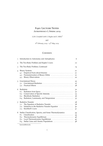
4.3. Binary Observationsd, we can then directly determine a as well (or both a1 and a2 if we see bothcomponents). The first known astrometric binary was the bright, northern starSirius – from its motion on the sky, astronomers first identified its tiny, faint,but massive white dwarf companion, Sirius b.More often, the data come from spectroscopic observations that measurethe stars’ Doppler shifts. If we can only measure the periodic velocity shiftsof one star (e.g. the other is too faint), then the “spectroscopic binary” is an“SB1”. If we can measure the Doppler shifts of both stars, then we have an“SB2”: we get the individual semimajor axes a1 and a2 of both components,and we can get the individual masses from m1 a1 m2 a2 .If we have an SB1, we measure the radial velocity of the visible star. Assuming a circular orbit, 2πt2πa1 sin Icos(3) vr1 PPwhere P and vr1 are the observed quantities. What good is a1 sin I? We knowthat a1 (m2 /M ) a, so from Kepler’s Third Law we see that (4)2πP 2 Gm32a31 M2Combining Eqs. 3 and 4, and throwing in an extra factor of sin3 I to eachside, we find(5)1G 2πP 2a3a sin3 I (6)1 v3r1G (2π/P)m32 sin3 IM2where this last term is the spectroscopic “mass function” – a single numberbuilt from observables that constrains the masses involved.(7)fm m32 sin3 I( m1 m2 )2In the limit that m1 m2 (e.g. a low-mass star or planet orbiting a moremassive star), then we have(8)f m m2 sin3 I m2Another way of writing this out in terms of the observed radial velocity semiamplitude K (see Lovis & Fischer 2010) is:(9)K 28.4 m s 1 m2 sin I(1 e2 )1/2 M Jup m1 m2M 2/3 P1 yr 1/3Fig. 2 shows the situation if the stars are eclipsing. In this example one staris substantially larger than the other; as the sizes become roughly equal (or as23

4. Binary SystemsFigure 2: Geometry of an eclipse (top), and the observed light curve (bottom).the impact parameter b reaches the edge of the eclipsed star), the transit looksless flat-bottomed and more and more V-shaped.If the orbits are roughly circular then the duration of the eclipse (T14 ) relates directly to the system geometry:(10) T14 2R1p1 (b/R1 )2v2while the fractional change in flux when one star blocks the other just scalesas the fractional area, ( R2 /R1 )2 .There are a lot of details to be modeled here: the proper shape of the lightcurve, a way to fit for the orbit’s eccentricity and orientation, also includingthe flux contribution during eclipse from the secondary star. Many of these details are simplified when considering extrasolar planets that transit their hoststars: most of these have roughly circular orbits, and the planets contributenegligible flux relative to the host star.Eclipses and spectroscopy together are very powerful: visible

number of stars per system is something like 1.6. Orbital periods range from 1day to 1010 days ( 3 106 yr). Any longer, and Galactic tides will disrupt the stable orbit (the Sun takes 200 Myr to orbit the Milky Way). The periods have a log-normal distribution – for Sun-like stars,