WIXLIB

4Sven Leyffer and Ashutosh MahajanSequential Quadratic Programming (SQP) Methods: SQP methods successively minimize aquadratic model, mk (d), subject to a linearization of the constraints about xk (Han, 1977; Powell, 1978; Boggs and Tolle, 1995) to obtain a displacement d : x xk .1minimize mk (d) : gkT d dT Hk d subject to ck ATk d 0, xk d 0,2d(3.1)where Hk ' 2 L(xk , yk ) approximates the Hessian of the Lagrangian and yk is the multiplierestimate at iteration k. The new iterate is xk 1 xk d, together with the multipliers yk 1 of thelinearized constraints of (3.1). If Hk is not positive definite on the null-space of the active constraintnormals, then the QP is nonconvex, and SQP methods seek a local minimum of (3.1). The solutionof the QP subproblem can become computationally expensive for large-scale problems because thenull-space method for solving QPs requires the factorization of a dense reduced-Hessian matrix.This bottleneck has led to the development of other methods that use LP solves in the local model,and these approaches are described next.Sequential Linear Programming (SLP) Methods: SLP methods construct a linear approximation to (1.1). In general, this LP will be unbounded, and SLP methods require the addition of atrust region (discussed in more detail in the next section):minimize mk (d) gkT d subject to ck ATk d 0, xk d 0, and kdk k ,d(3.2)where k 0 is the trust-region radius. Griffith and Stewart (1961) used this method without atrust region but with the assumption that the variables are bounded. In general, k 0 mustconverge to zero to ensure convergence. SLP methods can be viewed as steepest descent methodsand typically converge only linearly. If, however there are exactly n active and linearly independent constraint normals at the solution, then SLP reduces to Newton’s method for solving a squaresystem of nonlinear equations and converges superlinearly.Sequential Linear/Quadratic Programming (SLQP) Methods: SLQP methods combine the advantages of the SLP method (fast solution of the LP) and SQP methods (fast local convergence) byadding an equality-constrained QP to the SLP method (Fletcher and de la Maza, 1989; Chin andFletcher, 2003; Byrd et al., 2004). SLQP methods thus solve two subproblems: first,n an LP is solvedoto obtain a step for the next iteration and also an estimate of the active set Ak : i : [xk ]i dˆi 0from a solution dˆ of (3.2). This estimate of the active set is then used to construct an equalityconstrained QP (EQP), on the active constraints,1minimize qk (d) gkT d dT Hk d2dsubject to ck ATk d 0, [xk ]i di 0, i Ak .(3.3)If Hk is second-order sufficient (i.e., positive-definite on the null-space of the constraints), thenthe solution of (3.3) is equivalent to the following linear system obtained by applying the KKT

Nonlinear Constrained Optimization: Methods and Softwareconditions to the EQP: Hk T AkIkT Ak Ik xyA!5 gk Hk xk ck ,0where Ik [ei ]i Ak are the normals of the active inequality constraints. By taking a suitable basisfrom the LP simplex solve, SLQP methods can ensure that [Ak : Ik ] has full rank. Linear solverssuch as MA57 can also detect the inertia; and if Hk is not second-order sufficient, a multiple of theidentity can be added to Hk to ensure descent of the EQP step.Sequential Quadratic/Quadratic Programming (SQQP) Methods: SQQP methods have recentlybeen proposed as SQP types of methods (Gould and Robinson, 2010, 2008). First, a convex QPmodel constructed by using a positive-definite Hessian approximation is solved. The solution ofthis convex QP is followed by a reduced inequality constrained model or an EQP with the exactsecond derivative of the Lagrangian.Theory of Sequential Linear/Quadratic Programming Methods. If Hk is the exact Hessian ofthe Lagrangian and if the Jacobian of the active constraints has full rank, then SQP methods converge quadratically near a minimizer that satisfies a constraint qualification and a second-ordersufficient condition (Boggs and Tolle, 1995). It can also be shown that, under the additional assumption of strict complementarity, all four methods identify the optimal active set in a finitenumber of iterations.The methods described in this section are also often referred to as active-set methods, becausethe solution of each LP or QP provides not only a suitable new iterate but also an estimate of theactive set at the solution.3.2Interior-Point MethodsInterior-point methods (IPMs) are an alternative approach to active-set methods. Interior-pointmethods are a class of perturbed Newton methods that postpone the decision of which constraintsare active until the end of the iterative process. The most successful IPMs are primal-dual IPMs,which can be viewed as Newton’s method applied to the perturbed first-order conditions of (1.1): f (x) c(x)T y z 0 Fµ (x, y, z) (3.4)c(x) ,Xz µewhere µ 0 is the barrier parameter, X diag(x) is a diagonal matrix with x along its diagonal,and e (1, . . . , 1) is the vector of all ones. Note that, for µ 0, these conditions are equivalent tothe first-order conditions except for the absence of the nonnegativity constraints x, z 0.Interior-point methods start at an “interior” iterate x0 , z0 0 and generate a sequence of interior iterates xk , zk 0 by approximately solving the first-order conditions (3.4) for a decreasing

6Sven Leyffer and Ashutosh Mahajansequence of barrier parameters. Interior-point methods can be shown to be polynomial-time algorithms for convex NLPs; see, for example, (Nesterov and Nemirovskii, 1994).Newton’s method applied to the primal-dual system (3.4) around xk gives rise to the localmodel, Hk Ak I x T (3.5)00 y Fµ (xk , yk , zk ), AkZk0Xk zwhere Hk approximates the Hessian of the Lagrangian, 2 Lk , and the step (xk 1 , yk 1 , zk 1 ) (xk , yk , zk ) (αx x , αy y , αz z ) is safeguarded to ensure that xk 1 , zk 1 0 remain strictly positive.Relationship to Barrier Methods: Primal-dual interior-point methods are related to earlier barrier methods (Fiacco and McCormick, 1990). These methods were given much attention in the1960s but soon lost favor because of the ill-conditioning of the Hessian. They regained attentionin the 1980s after it was shown that these methods can provide polynomial-time algorithms forlinear programming problems. See the surveys (Wright, 1992; Forsgren et al., 2002) for furthermaterial. Barrier methods approximately solve a sequence of barrier problems,minimize f (x) µxnXlog(xi ) subject to c(x) 0,(3.6)i 1for a decreasing sequence of barrier parameters µ 0. The first-order conditions of (3.6) are givenby f (x) µX 1 e A(x)y 0 and c(x) 0.(3.7)Applying Newton’s method to this system of equations results in the following linear system:#!"! xHk µXk 2 Akgk µXk 1 e Ak yk .ATk0 yckIntroducing first-order multiplier estimates Z(xk ) : µXk 1 , which can be written as Z(xk )Xk µe, we obtain the system"#!!Hk Z(xk )Xk 1 Ak xgk µXk 1 e Ak yk ,Ak0 yckwhich is equivalent to the primal-dual Newton system (3.5), where we have eliminated z X 1 Z x Ze µX 1 e.Thus, the main difference between classical barrier methods and the primal-dual IPMs is that Zkis not free for barrier methods but is chosen as the primal multiplier Z(xk ) µXk 1 . This freedomin the primal-dual method avoids some difficulties with ill-conditioning of the barrier Hessian.

Nonlinear Constrained Optimization: Methods and Software7Convergence of Barrier Methods: If there exists a compact set of isolated local minimizers of(1.1) with at least one point in the closure of the strictly feasible set, then it follows that barriermethods converge to a local minimum (Wright, 1992).4Globalization Strategy: Convergence from Remote Starting PointsThe local improvement models of the preceding section guarantee convergence only in a smallneighborhood of a regular solution. Globalization strategies are concerned with ensuring convergence from remote starting points to stationary points (and should not be confused with globaloptimization). To ensure convergence from remote starting points, we must monitor the progressof the local method. Monitoring is easily done in unconstrained optimization, where we can measure progress by comparing objective values. In constrained optimization, however, we musttake the constraint violation into account. Three broad classes of strategies exist: augmented Lagrangian methods, penalty and merit-function methods, and filter and funnel methods.4.1Augmented Lagrangian MethodsThe augmented Lagrangian of (1.1) is given byρ(4.1)L(x, y, ρ) f (x) y T c(x) kc(x)k22 ,2where ρ 0 is the penalty parameter. The augmented Lagrangian is used in two modes to developalgorithms for solving (1.1): by defining a linearly constrained problem or by defining a boundconstrained problem.Linearly constrained Lagrangian methods: These methods successively minimize a shifted augmented Lagrangian subject to a linearization of the constraints. The shifted augmented Lagrangianis defined asρ(4.2)L(x, y, ρ) f (x) y T pk (x) kpk (x)k22 ,2where pk (x) are the higher-order nonlinear terms at the current iterate xk , that is,pk (x) c(x) ck ATk (x xk ).(4.3)This approach results in the following local model:minimize L(x, yk , ρk )xsubject to ck ATk (x xk ) 0, x 0.(4.4)We note that if ck ATk (x xk ) 0, then minimizing the shifted augmented Lagrangian is equivalent to minimizing the Lagrangian over these constraints. Linearly constrained, augmented Lagrangian methods solve a sequence of problems (4.4) for a fixed penalty parameter. Multipliersare updated by using a first-order multiplier update rule,yk 1 yk ρk c(xk 1 ),where xk 1 solves (4.4).(4.5)

8Sven Leyffer and Ashutosh MahajanBound-constrained Lagrangian methods: These methods approximately minimize the augmentedLagrangian,minimize L(x, yk , ρk ) subject to x 0.x(4.6)The advantage of this approach is that efficient methods for bound-constrained optimizationcan readily be applied, such as the gradient-projection conjugate-gradient approach (Moré andToraldo, 1991), which can be interpreted as an approximate Newton method on the active inequality constraints.Global convergence is promoted by defining two forcing sequences, ωk & 0, controlling the accuracy with which every bound-constrained problems is solved, and ηk & 0, controlling progresstoward feasibility of the nonlinear constraints. A typical bound-constrained Lagrangian methodcan then be stated as follows:Given an initial solution estimate (x0 , y0 ), and an initial penalty parameter ρ0 .while xk is not optimal doFind an ωk -optimal solution, xck of (4.6).if kc(xck )k ηk thenPerform a first-order multiplier update: yk 1 yk ρk c(xck )elseIncrease penalty: ρk 1 10ρkendSet k k 1endAlgorithm 2: Bound-Constrained Augmented Lagrangian Method.Theory of Augmented Lagrangian Methods. Conn et al. (1991) show that a bound-constrainedLagrangian method can globally converge if the sequence {xk } of iterates is bounded and if theJacobian of the constraints at all limit points of {xk } has column rank no smaller than m. Connet al. (1991) show that if some additional conditions are met, then their algorithm is R-linearlyconvergent. Bertsekas (1996) shows that the method converges Q-linearly if {ρk } is bounded,and superlinearly otherwise. Linearly constrained augmented Lagrangian methods can be madeglobally convergent by adding slack variables to deal with infeasible subproblems (Friedlanderand Saunders, 2005).4.2Penalty and Merit Function MethodsPenalty and merit functions combine the objective function and a measure of the constraint violation into a single function whose local minimizers correspond to local minimizers of the originalproblem (1.1). Convergence from remote starting points can then be ensured by forcing descent ofthe penalty or merit function, using one of the mechanisms of the next section.

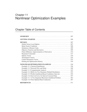
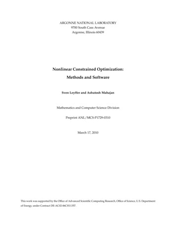
Nonlinear Constrained Optimization: Methods and Software9Exact penalty functions are an attractive alternative to augmented Lagrangians and are definedaspρ (x) f (x) ρkc(x)k,where ρ 0 is the penalty parameter. Most approaches use the 1 norm to define the penaltyfunction. It can be shown that a local minimizer, x , of pρ (x) is a local minimizer of problem (1.1)if ρ ky kD , where y are the corresponding Lagrange multipliers and k · kD is the dual norm ofk·k (i.e., the -norm in the case of the 1 exact-penalty function); see, for example, (Fletcher, 1987,Chapter 12.3). Classical approaches using pρ (x) have solved a sequence of penalty problems foran increasing sequence of penalty parameters. Modern approaches attempt to steer the penaltyparameter by comparing the predicted decrease in the constraint violation to the actual decreaseover a step.A number of other merit functions also exist. The oldest, the quadratic penalty function, f (x) ρkc(x)k22 , converges only if the penalty parameter diverges to infinity. Augmented Lagrangianfunctions and Lagrangian penalty functions such as f (x) y T c(x) ρkc(x)k have also been usedto promote global convergence. A key ingredient in any convergence analysis is to connect thelocal model to the merit function that is being used in a way that ensures a descent property of themerit function; see Section 5.1.4.3Filter and Funnel MethodsFilter and funnel methods provide an alternative to penalty methods that does not rely on the useof a penalty parameter. Both methods use step acceptance strategies that are closer to the originalproblem, by separating the constraints and the objective function.Filter methods: Filter methods keep a record of the constraint violation, hl : kc(xl )k, and objective function value, fl : f (xl ), for some previous iterates, xl , l Fk (Fletcher and Leyffer, 2002).A new point is acceptable if it improves either the objective function or the constraint violationcompared to all previous iterates. That is, x̂ is acceptable iff (x̂) fl γhlorh(x̂) βhl , l Fk ,where γ 0, 0 β 1, are constants that ensure that iterates cannot accumulate at infeasible limitpoints. A typical filter is shown in Figure 1 (left), where the straight lines correspond to the regionin the (h, f )-plane that is dominated by previous iterations and the dashed lines correspond to theenvelope defined by γ, β.The filter provides convergence only to a feasible limit because any infinite sequence of iteratesmust converge to a point, where h(x) 0, provided that f (x) is bounded below. To ensureconvergence to a local minimum, filter methods use a standard sufficient reduction conditionfrom unconstrained optimization,f (xk ) f (xk d) σmk (d),(4.7)

10Sven Leyffer and Ashutosh Mahajanwhere σ 0 is the fraction of predicted decrease and mk (d) is the model reduction from thelocal model. It makes sense to enforce this condition only if the model predicts a decrease in theobjective function. Thus, filter methods use the switching condition mk (d) γh2k to decide when(4.7) should be enforced. A new iterate that satisfies both conditions is called an f-type iterate,and an iterate for which the switching condition fails is called an h-type iterate to indicate that itmostly reduces the constraint violation. If a new point is accepted, then it is added to the currentiterate to the filter, Fk , if hk 0 or if it corresponds to an h-type iterations (which automaticallysatisfy hk 0).Funnel methods: The method of Gould and Toint (2010) can be viewed as a filter method withjust a single filter entry, corresponding to an upper bound on the constraint violation. Thus, thefilter contains only a single entry, (Uk , ). The upper bound is reduced during h-type iterations,to force the iterates toward feasibility; it is left unchanged during f-type iterations. Thus, it is possible to converge without reducing Uk to zero (consistent with the observation that SQP methodsconverge locally). A schematic interpretation of the funnel is given in Figure 1 (left).Figure 1: The left figure shows a filter where the blue/red area corresponds to the points that arerejected by the filter. The right figure shows a funnel around the feasible set.4.4Maratos Effect and Loss of Fast ConvergenceOne can construct simple examples showing that arbitrarily close to an isolated strict local minimizer, the Newton step will be rejected by the exact penalty function (Maratos, 1978), resultingin slow convergence. This phenomenon is known as the Maratos effect. It can be mitigated bycomputing a second-order correction step, which is a Newton step that uses the same linear system with an updated right-hand side (Fletcher, 1987; Nocedal and Wright, 1999). An alternativemethod to avoid the Maratos effect is the use of nonmonotone techniques that require descentover only the last M iterates, where M 1 is a constant.

Nonlinear Constrained Optimization: Methods and Software511Globalization MechanismsIn this section, we review two mechanisms to reduce the step that is computed by the local model:line-search methods and trust-region methods. Both mechanisms can be used in conjunction withany of the local models and any of the global convergence strategies, giving rise to a broad familyof algorithms. In Sections 7–9, we describe how these components are used in software for NCOs.5.1Line-Search MethodsLine-search methods enforce convergence with a backtracking line search along the direction s.For interior-point methods, the search direction, s ( x , y , z ), is obtained by solving theprimal-dual system (3.5). For SQP methods, the search direction is the solution of the QP (3.1), s d. It is important to ensure that the model produces a descent direction, e.g., Φ(xk )T s 0 for amerit or penalty function Φ(x); otherwise, the line search may not terminate. A popular line searchis the Armijo search (Nocedal and Wright, 1999), described in Algorithm 3 for a merit functionΦ(x). The algorithm can be shown to converge to a stationary point, detect unboundedness, orconverge to a point where there are no directions of descent.Given initial estimate x0 IRn , let 0 σ 1, and set k 0;while xk is not optimal doApproximately solve a local model of (1.1) around xk to find a search direction s.Make sure that s is a descent direction, e.g. Φ(xk )T s 0.Set α0 1 and l 0.repeatSet αl 1 αl /2 and evaluate Φ(xk αl 1 s). Set l l 1.until Φ(xk αl s) fk αl σsT Φk ;set k k 1.endAlgorithm 3: (Armijo) Line-Search Method for Nonlinear OptimizationLine-search methods for filters can be defined in a similar way. Instead of checking descent inthe merit function, a filter method is used to check acceptance to a filter. Unlike merit functions,filter methods do not have a simple definition of descent; hence, the line search is terminatedunsuccessfully once the step size αl becomes smaller than a constant. In this case, filter methodsswitch to a restoration step, obtained by solving a local approximation of (2.2).5.2Trust-Region MethodsTrust-region methods explicitly restrict the step that is computed by the local model, by addinga trust-region constraint of the form kdk k to the local model. Most methods use an norm trust region, which can be represented by bounds on the variables. The trust-region radius, k 0, is adjusted at every iteration depending on how well the local model agrees with the

12Sven Leyffer and Ashutosh MahajanNCO, (1.1).Given initial estimate x0 IRn , choose 0 0, and set k 0;while xk is not optimal doReset k ;repeatApproximately solve a local trust-region model with kdk k .if xk d is sufficiently better than xk thenAccept the step: xk 1 xk d; possibly increase k .elseReject the step and decrease the trust-region radius, e.g. k k /2.enduntil an improved solution estimate xk 1 is found ;Check whether xk 1 is optimal; set k k 1.endAlgorithm

2 Sven Leyffer and Ashutosh Mahajan In general, one cannot solve (1.1) directly or explicitly. Instead, an iterative method is used that solves a sequence of simpler, appr