Transcription
Adv Data Anal Classif (2015) 9:447–460DOI 10.1007/s11634-015-0220-zREGULAR ARTICLEImproved initialisation of model-based clustering usingGaussian hierarchical partitionsLuca Scrucca1 · Adrian E. Raftery2Received: 30 November 2014 / Revised: 3 October 2015 / Accepted: 12 October 2015 /Published online: 26 October 2015 Springer-Verlag Berlin Heidelberg 2015Abstract Initialisation of the EM algorithm in model-based clustering is often crucial. Various starting points in the parameter space often lead to different local maximaof the likelihood function and, so to different clustering partitions. Among the severalapproaches available in the literature, model-based agglomerative hierarchical clustering is used to provide initial partitions in the popular mclust R package. This choiceis computationally convenient and often yields good clustering partitions. However, incertain circumstances, poor initial partitions may cause the EM algorithm to convergeto a local maximum of the likelihood function. We propose several simple and fastrefinements based on data transformations and illustrate them through data examples.Keywords Model-based clustering · Model-based agglomerative hierarchicalclustering · mclust · Data transformationMathematics Subject Classificationcluster analysis)B62H30 (Classification and discrimination;Luca Scruccaluca@stat.unipg.itAdrian E. Rafteryraftery@u.washington.edu1Dipartimento di Economia, Università degli Studi di Perugia, Via A. Pascoli 20, 06123 Perugia,Italy2Department of Statistics, University of Washington, Box 354322, Seattle, Washington 98195-4322,USA123
448L. Scrucca, A. E. Raftery1 IntroductionModel-based clustering is an increasing popular method for unsupervised learning. Incontrast to classical heuristic methods, such as the original k-means proposal and hierarchical clustering, model-based clustering methods rely on a probabilistic assumptionabout the data distribution. According to the main underlying assumption, data aregenerated from a mixture distribution, where each cluster is described by one or moremixture components. Maximum likelihood estimation of parameters is usually carriedout via the EM algorithm (Dempster et al. 1977). The EM algorithm is an iterative,strictly hill-climbing procedure whose performance can be very sensitive to the starting point because the likelihood surface tends to have multiple modes, although itusually produces sensible results when started from reasonable starting values. Thus,good initialisation is crucial for finding MLEs, although no method suggested in theliterature uniformly outperforms the others.In the case of Gaussian model-based clustering (Fraley and Raftery 2002), severalapproaches are available, both stochastic and deterministic, for selecting an initial partition of the observations, or an initial estimate of the parameters. In the mclust Rpackage (Fraley et al. 2012, 2015), the EM algorithm is initialised using the partitionsobtained from model-based agglomerative hierarchical clustering. Efficient numericalalgorithms exist for approximately maximising the classification likelihood with multivariate normal models. However, in certain circumstances, poor initial partitions maycause the EM algorithm to converge to a local maximum of the likelihood function.In this contribution we discuss cases where an initial partition may lead to suboptimal maximum likelihood estimates when applied to coarse data with ties (e.g.discrete data or continuous data that are rounded in some form when measured), and wepresent some possible refinements to improve the fitting of such finite mixture models.The outline of this article is as follows. Section 2 gives a brief review of background material on model-based clustering, with special attention devoted to some ofthe proposals available in the literature for the initialisation of EM algorithm. Section 3 discusses the model-based hierarchical agglomerative clustering method usedfor starting the EM algorithm. This is a very convenient and efficient algorithm, butin certain circumstances presents a serious drawback. Section 4 contains some simple transformation-based methods to refine the EM initialisation step derived frommodel-based agglomerative hierarchical clustering. The behaviour of these methodsis illustrated through the use of real data examples in Sect. 5. The final section providessome concluding remarks.2 Background2.1 Model-based clustering overviewLet x 1 , x 2 , . . . , x n be a sample of n independent identically distributed observations.The distribution of every observation is specified by a probability mass or densityfunction through a finite mixture model of G components, which takes the followingform123
Improved initialisation of model-based clustering.f (x; ) G 449πk f k (x; θ k ),(1)k 1where {π1 , . . . , πG 1 , θ 1 , . . . , θ G } are the parameters of the mixture model,f k (x; θ k ) is the kth component density at x with parameter(s) G θ k , (π1 , . . . , πG 1 ) areπk 1), and G is thethe mixing weights or probabilities (such that πk 0, k 1number of mixture components.Assuming G fixed, mixture model parameters are usually unknown and mustbe estimated. The log-likelihoodfunction corresponding to Eq. (1) is given by nlog( f (x i ; )). Direct maximisation of the log-likelihood ( ; x 1 , . . . , x n ) i 1function is often complicated, so MLE of finite mixture models is usually carried outvia the EM algorithm (McLachlan and Peel 2000).In the model-based approach to clustering, each component of a finite mixture ofdensity functions belonging to a given parametric class is associated with a groupor cluster. Most applications assume that all component densities arise from thesame parametric distribution family, although this need not be the case in general. A popular model assumes a Gaussian distribution for each component, i.e.f k (x; θ k ) N (μk , k ). Thus, clusters are ellipsoidal, centred at the mean vector μk ,and with other geometric features, such as volume, shape and orientation, determinedby k . Parsimonious parameterisations of the covariance matrices can be defined bymeans of eigen-decomposition in the form k γk O k Ak O k , where γk is a scalarcontrolling the volume of the ellipsoid, Ak is a diagonal matrix specifying the shapeof the density contours, and O k is an orthogonal matrix which determines the orientation of the corresponding ellipsoid (Banfield and Raftery 1993; Celeux and Govaert1995). Fraley et al. (2012, Table 1) summarized some parameterisations of withingroup covariance matrices available in the mclust software, and the correspondinggeometric characteristics.The number of mixture components and the parameterisation of the componentcovariance matrices can be selected on the basis of model selection criteria, such asthe Bayesian information criterion (BIC; Schwartz 1978; Fraley and Raftery 1998) orthe integrated complete-data likelihood criterion (ICL; Biernacki et al. 2000).2.2 Initialisation of EM algorithmThe EM algorithm is an easy to implement, numerically stable algorithm, which has,under fairly general conditions, reliable global convergence. However, it may convergeslowly and, like any other Newton-type method, does not guarantee convergence to theglobal maximum when there are multiple maxima (McLachlan and Krishnan 2008,p. 29). Further, in the case of finite mixture modelling, the estimates obtained dependon the starting values. Thus initialisation of EM is crucial because the likelihoodsurface tends to have multiple modes, although it usually produces sensible resultswhen started from reasonable starting values (Wu 1983; Everitt et al. 2011, p. 150).Several approaches are available, both stochastic and deterministic, for initialisingthe EM algorithm. Broadly speaking, there are two general approaches. The first onestarts from some initial values for the parameters to be estimated. A simple strategy123
450L. Scrucca, A. E. Rafteryis based on generating several candidates by drawing parameter values uniformly atrandom over the feasible parameters regions. Since the random-starts strategy hasa fair chance of not providing good initial starting values, a common suggestion toalleviate this problem is to run the EM algorithm with several random starts and tochoose the best solution. However, such a strategy can be quite time consuming andis not always practical, especially for high-dimensional datasets.Two other stochastic initialisation schemes are the so-called emEM and rndEM. Theformer approach, proposed by Biernacki et al. (2003), uses several short runs of theEM initialised with valid random starts as parameter estimates until an overall numberof total iterations is exhausted. Then, the solution with the highest log-likelihood ischosen to be the initialiser for the long EM, which runs until the usual strict convergencecriteria are met. This approach is computationally intensive and the same commentsmade above about random starts apply to it also.Two related approaches were proposed by Maitra (2009), one called Rnd-EM wherethe short EM stage is replaced by choosing multiple starting points and evaluatingthe log-likelihood at these values without running any EM iterations. Then, the bestobtained solution serves as an initialiser for the long EM stage. The second proposal isa staged approach based on finding a large number of local modes of the dataset, andthen to choose representatives from the most widely-separated ones. This approachis reported to be very time-consuming for high-dimensional data, and Melnykov andMaitra (2010) found the method to be outperformed by emEM and RndEM. Recently,Melnykov and Melnykov (2012) have proposed a strategy for initialising mean vectorsby choosing points with higher concentrations of neighbours and using a truncatednormal distribution for the preliminary estimation of dispersion matrices.A second kind of approach for initialising the EM algorithm is based on the partitionobtained from another clustering algorithm, e.g. k-means or hierarchical agglomerative clustering (HAC). In this case, the final classification is used to start the EMalgorithm from the M-step. Unfortunately, most of these partitioning algorithm haveseveral drawbacks, such as the need to be properly initialised or the tendency to imposespecific shapes and patterns on clusters. In the popular mclust package for R, theEM algorithm is initialised using the partitions obtained from model-based hierarchical agglomerative clustering (MBHAC). In this approach, k clusters are obtainedfrom a large number of smaller clusters by recursively merging the two clusters thathave the smallest dissimilarity in a model-based sense, i.e. the dissimilarity used foragglomeration is derived from a probabilistic model. Banfield and Raftery (1993)proposed a dissimilarity based on a Gaussian mixture model, which is equal to thedecrease in likelihood resulting by the merging of two clusters. Fraley (1998) showedhow the structure of some specific Gaussian models can be exploited to yield efficientalgorithms for agglomerative hierarchical clustering. More details about this approachare discussed in the following section.3 Model-based hierarchical agglomerative clusteringThe objective of MBHAC is to obtain a hierarchical ordering of clusters of n objectson the basis of the some measure of similarity among them. The result is a tree-123
Improved initialisation of model-based clustering.451like structure, which proceeds from n clusters containing one object to one clustercontaining all n objects by successively merging objects and clusters.Given n objects or observations (x 1 , . . . , x n ), let (z 1 , . . . , z n ) denote the classification labels, i.e. z i k if x i is assigned to cluster k. The unknown parameters areobtained by maximising the classification likelihoodLC (θ 1 , . . . , θ G , z 1 , . . . , z n x 1 , . . . , x n ) n f zi (x i θ zi ).i 1Assuming the multivariate Gaussian distribution for f k (x i θ k ), the parameters arethe mean vector μk and the covariance matrix k . By imposing different covariancestructures over k , different criterion can be derived (see Fraley 1998). For instance,when the covariance is allowed to be different among clusters, the criterion to beminimised at each hierarchical stage isWG G k 1 Wk , n k log nk (2)where n k is the number of observations in group k and W k is the sample crossproduct matrix for the kth group (k 1, . . . , G). Efficient numerical algorithms areavailable for approximately maximising the classification likelihood (or, equivalently,minimising the corresponding criterion) with multivariate Gaussian models have beendiscussed.As mentioned, the above MBHAC approach is used for starting the EM algorithmin the mclust R package. This is particularly convenient because the underlyingprobabilistic model can be shared by the initialisation step and the model fitting step.MBHAC is also computationally convenient because a single run provides the basisfor initialising the EM algorithm for any number of mixture components and parameterisations of the component covariance matrices.However, a serious problem for the MBHAC approach may arise when, at anystage, two pairs of objects attain the same minimum value for the criterion in (2).In the presence of coarse data, resulting from the discrete nature of the data or fromcontinuous data that are rounded in some way when measured, ties must be brokenby choosing the pair of entities that will be merged. This is often done at random but,regardless of which method is adopted for breaking ties, this choice can have importantconsequences because it changes the clustering of the remaining observations. In thiscase the final EM solution may depend on the ordering of the variables, and to a lesserextent on permutation of the observations (the latter case is not studied further in thispaper).This difficulty is known as the ties in proximity problem in the hierarchical clusteringliterature (see, for example, Jain and Dubes 1988, Sec. 3.2.6). This problem can alsoarise in other contexts, such as k-means clustering (Gordon 1999, p. 42) or partitionaround medoids (PAM; Kaufman and Rousseeuw 1990, p. 104).123
452L. Scrucca, A. E. Raftery4 Transformation-based approaches for obtaining starting partitions inmodel-based hierarchical agglomerative clusteringIn this section we describe some simple proposals for starting the EM algorithm usingthe partitions obtained with MBHAC. Ideally, we would like to retain the positiveaspects of such approach, but, at the same time, reduce the chance that a poor initialpartition causes the EM algorithm to converge to a local maximum of the likelihoodfunction.The idea is to project the data through a suitable transformation before applying theMBHAC at the initialisation step. Once a reasonable hierarchical partition is obtained,the EM algorithm is run using the data on the original scale.Let X be the (n p) data matrix, and X (X 1n x̄ ) be the correspondingcentred matrix, where x̄ (x̄1 , . . . , x̄ p ) is the vector of sample means, and 1n is the {si j } X X/n be the ( p p) sample covarianceunit vector of length n. Let matrix. Consider the singular value decomposition (SVD) of the centred data matrix,X U DV r λi ui v i ,i 1where ui are the right singular vectors, v i the left singular vectors, λ1 λ2 . . . λr 0 the singular values, and r the rank of matrix X. Similarly, the centred andscaled data matrix can be decomposed asXS 1/2 U D V r λi ui v i ,i 1where S diag(s12 , . . . , s 2p ) is the diagonal matrix of sample variances. In both SVDdecompositions the rank r is the rank of the data matrix, i.e. r min(n, p), withequality when there are no singularities.We now provide the details of the transformations investigated and some remarks.4.1 Data spheringSphering (or whitening) the data (SPH) is obtained by applying the following transformation: Z SPH XV D 1 n U n, where V and D 1 n diag( n/λi ) are, respectively, the matrix of eigenvectorsand the diagonal matrix of square root inverse of eigenvalues from the spectral decom For this transformation, E(Z SPH ) 0position of the sample marginal covariance, .and Var(Z SPH ) I, so the features are centred at zero, with unit variances and uncorrelated. Thus, this transformation converts an elliptically shaped symmetric cloud ofpoints into a spherically shaped cloud.123
Improved initialisation of model-based clustering.4534.2 PCA scores from covariance matrixThe principal component transformation from the covariance matrix (PCS) is obtainedas:Z PCS XV U D,for which E(Z PCS ) 0 and Var(Z PCS ) D2 /n diag(λi2 /n), so the features are centred, uncorrelated and with decreasing variances equal to the eigenvalues of .Usually the first few components account for most of the dispersion in the data. Asimilar idea was proposed by McLachlan (1988), who discussed the use of principalcomponent analysis in a preliminary exploratory analysis for the selection of suitablestarting values.4.3 PCA scores from correlation matrixThe principal component transformation from the correlation matrix (PCR) is definedas:Z PCR XS 1/2 V U D ,for which E(Z PCR ) 0 and Var(Z PCR ) D 2 /n diag(λi 2 /n), so the features arecentred, uncorrelated and with decreasing variances equal to the eigenvalues of the S 1/2 .marginal sample correlation matrix, S 1/2 4.4 Scaled SVD projectionThe scaled SVD transformation (SVD) is computed as:Z SVD XS 1/2 V D 1/2 U D 1/2 ,for which E(Z SVD ) 0 and Var(Z SVD ) D /n diag(λi /n). Again the featuresare centred, uncorrelated and with decreasing variances equal to the square root of the S 1/2 . In this case theeigenvalues of the marginal sample correlation matrix, S 1/2 features’ dispersion presents a gentle decline compared to the PCR case.4.5 RemarksAll the above transformations allow one to remove the “ordering” effect, so that evenin the presence of ties the partitions obtained by applying MBHAC are invariant topermutations of the input variables. Furthermore, as shown in the next section throughexamples with real data, most of them allow one to achieve better clustering resultswhen used for initialising the EM algorithm in Gaussian model-based clustering.To get an idea of this, consider Fig. 1 where we report a scatterplot matrix with pairsof plots for the original variables in the Crabs dataset (to be discussed in Sect. 5.1) and123
454L. Scrucca, A. E. Raftery 0.4 0.1 0.1 0.3 0.3 0.10.1 0.20.00.2 0.10 0.000.100.0 0.5SVD1 0.1 0.1 0.3 1.0FL101520SVD20.1 0.4RW 0.3 0.1101520SVD3CL100.20.01520SVD4 0.2CW101520SVD5BD101520101520101520101520Fig. 1 Scatterplot matrix for the Crabs data: lower panels show scatterplots for pairs of variables in theoriginal scale; upper panels show the features obtained by applying the scaled SVD transformation. For allgraphs points are marked according to the true classesfor scaled SVD-transformed features in, respectively, the lower and upper panels, andwith points marked according to the true classes. In the graphs for the variables in theoriginal scale is hard to detect any clustering structure, whereas in the first three SVDfeatures there appears to be a certain degree of separation among classes. ApplyingMBHAC on this features space should provide better starting points for applying theEM algorithm.5 Data analysesIn this section we present some examples using real data. We compare the behaviourof the proposed transformations against the usual MBHAC for starting the EM algorithm, and two common strategies for GMMs initialisation. The first strategy is to startfrom the best partition obtained out of 50 runs of the k-means algorithm. The secondis the emEM strategy as implemented in the mixmod software (Biernacki et al. 2006;123
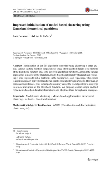
Improved initialisation of model-based clustering.455Auder et al. 2014), which, by default, uses 50 short runs of EM, each made of 5 iterations, followed by a long run of EM from the solution maximising the log-likelihood.The tolerance used for assessing the log-likelihood relative convergence of the EMalgorithm is set to 10 5 .The comparison among the different initialising strategies is based on two measures,the BIC and the adjusted Rand index (ARI). The former is used to select the bestGaussian finite mixture model with respect to both the number of components and thecomponent-covariances decomposition. The BIC for model M with k componentshas the following form x) νM,k log(n),BICM,k 2 ( ; x) is the maximised log-likelihood, νM,k is the number of independentwhere ( ;parameters to be estimated in model M, and k is the number of mixture components.This criterion depends on the starting partition through the log-likelihood at the MLEs penalised by the complexity of the model. It is the default criterion used in mclust ,for selecting a model, so the larger the value of the BIC the stronger the evidence forthe corresponding model and number of components.The ARI (Hubert and Arabie 1985) is used for evaluating the clustering obtainedwith a given mixture model. This is a measure of agreement between two partitions,one estimated by a statistical procedure independent of the labelling of the groups,and one being the true classification. The ARI has zero expected value in the case of arandom partition, and it is bounded above by 1, with higher values representing betterpartition accuracy. Furthermore, it can be applied to compare partitions having differentnumbers of parts. The ARI is the index recommended by Milligan and Cooper (1986)for measuring the agreement between an external reference partition and a clusteringpartition. In the following data analysis examples, we take advantage of the knowledgeof the true classes for measuring clustering accuracy, but not for model fitting.5.1 Crabs dataWe now consider a dataset consisting of data on five morphological measurements for200 Leptograpsus crabs, with 50 crabs for each of two colour forms (blue and orange)and both sexes. Figure 2 shows the marginal distribution for each variable. In eachstripchart data points are stacked to avoid overlapping, so the presence of several tiesin the data is evident.Overall, there are 5! 120 possible different ordering of the variables, of which 105lead to selection of the (EEE,9) model, and 15 the (EEV,3) model. Table 1 shows thecorresponding BIC and ARI obtained for these models and for models initialised usingthe transformations discussed in Sect. 4. As it can be seen, initialisation with the scaledSVD transformation returns the model with both the largest BIC and the most accuratepartition (ARI 0.7938). This transformation is the only one that selects the correctnumber of mixture components. Initialisation based on k-means also yields the rightnumber of components, but its fit and accuracy are substantially worse. The emEMinitialisation strategy yields a better fit, but it selects the wrong number of clusters.123
456L. Scrucca, A. E. 0304050BD101520Fig. 2 Stripcharts with stacked data points for the Crabs data showing the marginal distribution for eachvariable. From this plot the presence of several ties is clearly visibleTable 1 Results from different initialisation strategies for the Crabs dataInitialisationMkBICARISystem time (s)MBHACDefault(105)EEE9 2883.680.48312.61(15)EEV3 2925.590.47152.47SPHEEE8 2861.270.52482.40PCSEEE9 2883.680.48312.69PCREEE10 2894.650.45722.72SVDEEV4 2842.300.79381.88k-meansEEV4 2916.680.59262.78emEMEEE6 2866.610.630511.08All possible orderings of the variables are reported for the default MBHAC initialisation; values amongparentheses provide the number of such orderings which converge to the same solution. Larger values ofboth BIC and ARI are better. The best values are shown in bold font. System times are averaged over 10runs of the estimation algorithmRaftery and Dean (2006) selected as optimal subset for clustering purposes thevariables (FL, RW, CW, BD) (in the identified ordering). Also for such a subset,different orderings give different results in 7 out of 24 possible arrangements. Table 2123
Improved initialisation of model-based clustering.457Table 2 Results from different initialisation strategies for the Crabs data using the optimal subset ofvariables identified by Raftery and Dean (2006)InitialisationMkBICARISystem time (s)MBHACDefault(17)EEV4 2609.890.81542.54(5)EEV5 2645.190.74872.40(1)EEV4 2609.900.82762.40(1)EEE11 2674.400.41062.46SPHEEV4 2609.790.81541.89PCSEEV4 2609.890.81542.55PCREEE8 2652.580.48602.52SVDEEV4 2609.780.84002.06k-meansEEE5 2661.070.56082.62emEMEEV4 2609.870.81548.70All possible orderings of the variables are reported for the default MBHAC initialisation; values amongparentheses provide the number of such orderings which converge to the same solution. Larger values ofboth BIC and ARI are better. The best values are shown in bold font. System times are averaged over 10runs of the estimation algorithmshows the clustering results obtained with different initialisation strategies using theabove mentioned optimal subset of variables. Again, initialisation with the scaledSVD transformation yields the largest BIC and the highest ARI among the consideredstrategies, with a slight improvement over the default initialisation with the identifiedordering of the variables. Note that emEM has results analogous to the best defaultMBHAC initialisation, but k-means results are markedly worse.Finally, note that, using both the full set of the variables and the optimal subset, analysis with the initialisation using the scaled SVD transformation used thesmallest computing time. This may appear counterintuitive at first sight, becausecomputing the SVD is time consuming. However, this is more than balanced by thefact that having good starting values allows the EM algorithm to converge in fewersteps.5.2 Female voles dataFlury (1997) reported the data for a sample of 86 female voles from two species,41 from Microtus californicus and 45 from Microtus ochrogaster, and seven variablesdescribing various body measurements in units of 0.1mm, so several ties are containedin this data set.There are 7! 5040 possible orderings of the variables. When the default initialisation is used, there is considerable variation among the resulting solutions: 41 finalmodels with different BIC values (up to 5 significant digits) are estimated, leading to38 different partitions. From Table 3, about 67 % of the solutions give a single compo-123
458L. Scrucca, A. E. RafteryTable 3 Results from different initialisation strategies for the female voles dataInitialisationMKBICARISystem time (s)MBHACDefault(3395)XXX1 3874.90.00000.19(996)EEE3 3862.80.77200.29(381)EEE2 3844.20.90810.23(253)EEE4 3872.60.60150.24SPHEEE5 3871.00.41290.26PCSXXX1 3874.90.00000.22PCREEE2 3844.20.90810.22SVDEEE2 3844.20.90810.19k-meansEEE4 3872.60.60150.25emEMEEE2 3844.20.90812.43The results for the default MBHAC initialisation are reported for some of all possible orderings of thevariables; values among parentheses provide the number of such orderings which converge to the same pair(M, k). Larger values of both BIC and ARI are better. The best values are shown in bold font. Systemtimes are averaged over 10 runs of the estimation algorithmnent model, about 20 % have three components, and only about 7.5 % of the solutionscorrectly identify the correct number of clusters. On the contrary, three transformationbased initialisation strategies are able to achieve the best fit in term of BIC, which inturn provides the largest ARI. The same optimal solution is also achieved by the emEMstrategy, whereas results from the k-means initialisation are inferior. Note that also inthis case the scaled SVD transformation is among the best strategies, with no increasein computing time.5.3 Italian wines dataForina et al. (1986) reported data on several chemical and physical properties of 178wines grown in the same region in Italy but derived from three different cultivars(Barolo, Grignolino, Barbera). We consider 27 of the original 28 variables that weredescribed in the Forina et al. paper and are available in the pgmm R package (McNicholas et al. 2015). In what follows, the data are analysed on the standardised scaleand, given the large number of features, only the common full covariance matrix model(EEE) is examined. Table 4 shows the results obtained using different MBHAC initial partitions, k-means and emEM initialisation strategies. Except for one case, theMBHAC initialisations allow one to achieve good clustering accuracy. In particular,SVD has the highest BIC and attains a clustering that perfectly matches the real classes.By comparison, the models initialised by k-means and emEM show somewhat worsevalues of both BIC and ARI.123
Improved initialisation of model-based clustering.459Table 4 Results from different initialisation strategies for the Italian wines dataInitialisationMKBICARISystem time (s)MBHACDefaultEEE3 12309.900.94890.36SPHEEE2 12370.800.58200.78PCSEEE3 12309.900.94890.36PCREEE3 12309.900.94890.37SVDEEE3 12306.751.00000.35k-meansEEE3 12314.720.96370.74emEMEEE4 12312.040.83553.99Larger values of both BIC and ARI are better. The best values are shown in bold font. System times areaveraged over 10 runs of the estimation algorithm6 Final commentsThe mixture model-based approach to clustering provides a firm statistical framework for unsupervised learning. The EM algorithm is typically used for parameterestimation. However, because of the many local maxima of the likelihood function,an important problem for getting sensible maximum likelihood estimates is to obtainreasonable starting points. A computationally efficient approach to EM initialisationis based on the partitions obtained from agglomerative hierarchical clustering.In this paper we h
same parametric distribution family, although this need not be the case in gen- . Fraley et al. (2012, Table 1) summarized some parameterisations of within- . The result is a tree-123. Improved initialisa