Transcription
Chapter 4: Modeling of gravity attraction214. Modeling of Gravity Attraction4.1. Gravity Anomalies of Bodies with Simple GeometricShapesTo appreciate the contributions of complex-shaped bodies to gravity anomalies, it ishelpful to understand the gravitational effects of bodies with simple geometric shapes.In the following chapter computer programs for the computation of the verticalgravitational effect of simple shaped bodies are presented using the software packageMATLAB (Hanselman and Littlefield, 1995).Throughout the chapter the following notations are used:- gz vertical gravitational effect of the body- ρ density contrast- G gravitational constant.4.1.1. Vertical gravitational attraction of a sphereThe attraction of sphere buried below earth's surface can be viewed in much the sameas the attraction of the entire earth from some distance in space; the formula ofvertical gravity effect at point P (fig. 4.1a) is (Telford et al., 1981): g z 4πG ρR 3z3x2 z2((4.1))3/ 2where:R radius of sphere (m)x horizontal distance from the centre (m)z depth of sphere (m)PxθrzR gzρ2 -ρ1 ρρ2ρ1Fig. 4.1a Vertical gravity effect of a sphere at point P.The change of the vertical gravity effect gz with ρ 1000 kg/m3, R 1 m and z 1m, 1.1 m and 1.2 m is shown in figure 4.1b; the name of the program isgrav sphere.m (appendix A.1).
Chapter 4: Modeling of gravity attraction gz gz gz22Fig. 4.1b Vertical gravity effect of a sphere with ρ 1000kg/m3, R 1 m and z 1, 1.1, 1.2 m.4.1.2. Vertical gravitational attraction of a thin rodThe vertical gravitational attraction gz of a thin rod with an inclination α and crosssection A at point P (fig.4.2a) is (Telford, 1981): g z G ρ A x z cot αx z cot α L cos α 2 1/21/222x sin α (z csc 2 α 2 xz cot α x 2 ) ()()Lzcscαx2xLcosαzcotα {}. (4.2)where: A cross-section [m2]x horizontal distance from O [m]z depth of top thin rod [m]α inclinationL length of thin rod [m]The change of gz for a thin rod with inclination α 45o, 90o, 135o, z 1 m, ρ 1000 kg/m3, A 1 m2, L 100 m is shown in figure 4.2b; the name of the program isgrav thin rod.m (appendix A.2).
Chapter 4: Modeling of gravity attraction23OPxαθzr gzdllLFig. 4.2a Vertical gravity effect of a thin rod at point P.8x 10-3Vertical Gravity Effect of Dipping Thin Rod135 45 790 6 gz (mgal)543210-10-8-6-4-20x (m)246810Fig. 4.2b Vertical gravity effect gz of a thin rod dipping with inclination α 45o, 90o, 135o, z 1 m, ρ 1000 kg/m3, A 1 m2, L 100 m.
Chapter 4: Modeling of gravity attraction244.1.3. Vertical gravitational attraction of vertical rectangular prismof cross section AThe vertical gravity effect gz at point P produced by a prism of cross section A(side small compared to distance to prism axis) (fig. 4.3a) extending from depth h1 toh2 is (Dehlinger, 1978): g z G(x ρ A2 y)2 1/ 2(cos α1 cos α 2 )(4.3a)or 1 g z G ρ A x2 y 2 h21 ()1/ 2 1/ 2 x 2 y 2 h22 1()(4.3b)where: A cross-section [m2]x,y horizontal distance from P to prism [m]h1 depth of prism top [m]h2 depth of prism bottom [m]P(0,0,0)xxα1yα2r1x, y,h1r2yzx, y,h2Fig. 4.3a Vertical gravity effect gz of a rectangular prism which cross-section A at point P.The change of the vertical gravity effect gz of a vertical rectangular prism with depthh1 1 m and h2 100 m, ρ 1 g/cm3, A 1 m2 (V 99 m3) dependent on x and yis shown in fig. 4.3b; the name of the program is grav prism.m (appendix A.3).
Chapter 4: Modeling of gravity attraction gz25Fig. 4.3b Vertical gravity effect gz of a prism with depth h1 1 m and h2 100 m, ρ 1000kg /m3, A 1 m2.4.1.4. Vertical gravitational attraction of vertical rectangularparallelepipedThe shape of an irregular three-dimensional body can be approximated by rectangularparallelepipeds, especially cubes. The vertical gravity effect gz of a parallelepipedproduced at a corner P of the body with sides x, y and z (fig. 4.4a) is (Talwani, 1973): π g z G ρ z 1 sin 1 (cos β cos λ ) sin 1 (cos β sin λ ) 2x (r y1 )(rz y1 ) y1 (r1 x1 )(rz x1 ) 1 ln 1 ln 2 (r1 y1 )(rz y1 ) 2 (r1 x1 )(rz x1 ) where:r1 (x12 y12 z12 )1/2rx (y12 z12 )1/2 ry (x12 z12 )1/2cos l x1/r1cos m y1/r1cos α z1/rxcos β z1/ryrz (x12 y12 )1/2cos n z1/r1cos λ y1/rz(4.4)sin λ x1/rzThis equation can be applied successively to compute the vertical gravity effect of aparallelepiped where P is not at a corner (fig. 4.4b).
Chapter 4: Modeling of gravity z2)J(x2,y2,z2)K(x2,y2,z2)z(a)(b)Fig. 4.4 Bodies for computing vertical gravity effect at P: (a). rectangular parallelepiped with onecorner at origin of coordinates, (b). rectangular parallelepipeds; the shaded parallelepiped does not havecorner at the origin.The vertical gravity effect of the rectangular parallelepiped CK is the sum anddifference of eight rectangular parallelepipeds, whereby seven have a corner at P(Talwani, 1973). Thus:( g)CK ( g)PK - ( g)PJ ( g)PG - ( g)PH - ( g)PF ( g)PE - ( g)PC ( g)PD(4.5)Fig. 4.4c shows the change of vertical gravity effect gz of such a general rectangularparallelepiped. The parameters are z1 1 m, z2 2 m, x2 – x1 1 m, y2 – y1 1 m (V 1 m3); the horizontal distances of x1, x2, y1, y2 are varying toward the origin, ρ 1000 kg/m3. The name of the program is grav rectangular.m (appendix A.4).
Chapter 4: Modeling of gravity attraction gz27Fig. 4.4c Vertical gravity effect of rectangular parallelepiped with none corner at the origin; z1 1 m,z2 2 m, x2 – x1 1 m, y2 – y1 1 m; the horizontal distances of x1, x2, y1, y2 are varying toward origin, ρ 1000 kg/m3.4.1.5. Vertical gravitational attraction of thick vertical cylinderThe vertical gravity effect gz at a point P on the axis of a vertical cylinder (fig. 4.5a)is (Telford et al., 1981):2 g z 2 πG ρ L z 2 R 2 ( z L ) R 2 (4.6a) where:R radius of cylinder (m); z depth of cylinder (m); L length of cylinder (m).Pr2r1zPθLLR(a)(b)Fig. 4.5 (a) Vertical gravity effect gz of a vertical cylinder on the axis; (b) of cylindrical slice.
Chapter 4: Modeling of gravity attraction28There are several significant limiting cases of this formula.1. If R , we obtain the infinite horizontal slab (Bouguer plate of thickness L): g z 2 πG ρL(4.6b)2. The vertical gravitational effect gz of a sector of the cylinder (fig. 4.4b) is:)( g z G ρθ r12 L2 r22 L2 (r2 r1 )(4.6c)where:r1 inner radius (m)r2 outer radius (m)θ sector angle (radian)This is the formula of the terrain correction (see 3.2.4), where L - the depth of thesector - corresponds to the difference between the height of the station and theaverage elevation in the sector.3. If z 0, the cylinder outcrops:( g z 2πG ρ L R L2 R 2)(4.6d)4. If L , equation 4.6a becomes:( g z 2πG ρ z 2 R 2 z)(4.6e)When L z, (that means the cylinder length is considerably larger than the depth zof the top of the cylinder), equation 4.6e can be used to compute the gravity effect fora station P off-axis using the well-known methods of solving Laplace's equation.Since gz satisfies Laplace's equation, gz can be expressed for r z R in a series ofLegendre polynomials of the form (fig. 4.6a): g z (r ,θ) k bn r (n 1) Pn (cos θ)n 0where:k 2πG ρbn coefficientsPn(cos θ) Legendre polynomialsr2 x2 z2tan θ x/z(4.7)
Chapter 4: Modeling of gravity attraction29xOzPθrRL zFig. 4.6a Vertical gravity effect of the thick vertical cylinder at an arbitrary point P.On the axis θ 0, r z, the series reduces to b P b P b P b P g z 2πG ρ 0 0 1 2 1 2 3 2 3 4 3 . zzz z bbb b 2πG ρ 0 12 23 34 . zz z z(4.8)where:P0, P1, P2, . 1 (Legendre polynomials for θ 0).This result must be the same as that given by equation 4.6e; expanding this equationin terms of R/Z with binomial series equation (4.8) becomes R2 g z 2πG ρ z 1 2 z z (4.9) R2 R4 R65R 87 R 10 2πG ρ 3 . 16 z 5 128 z 7 256 z 9 2z 8z Equating the coefficients of the two series (equations 4.8 and 4.9) deliversbn 0, if n is odd, andb0 R2R4R65R87 R 10, b2 , b4 , b6 , b8 .2816128256The expression gz(r,θ) for an off-axis point P is then
Chapter 4: Modeling of gravity attraction305 1 R 1 R 31 R g z (r , θ) 2 πG ρR P2 (cos θ) P4 (cos θ) 2 r 8 r 16 r 79 5 R 7 R P6 (cos θ) P8 (cos θ) L 128 r 256 r (4.10)Equation 4.10 can be rewritten to resemble equation 4.2 for the long thin rod. Byinserting r x 2 y 2 , gz(r,θ) can be expressed as 1 g z (r , θ ) πG ρR 2 x2 z2 ()12 R 2 P2 (cos θ )(4 x z2)32 2 R 4 P4 (cos θ)(8 x z2)52 2 (4.11) 5 R P6 (cos θ) 7 R P6 (cos θ) L 79 64 x 2 z 2 2 128 x 2 z 2 2 6(8)()This equation gives more precise results then equation 4.2, when the rod is vertical,although the difference between the two solutions is negligible, if z 2R.A more useful result for the same thick cylinder can be developed when z R:expanding equation 4.6e in terms of z/R rather than R/z: z2 g z 2 πG ρ R 1 2 z R (4.12)2 zzz4z65z 87 z 10 2 πG ρR 1 L R 2 R 2 8 R 4 16 R 6 128 R 8 256 R 10 Within the interval z r R the series is developed to an off-axis series: g z (r ,θ) k a m r m Pm (cos θ)m 0() k a0 a1 rP1 (cos θ) a 2 r P2 (cos θ) a 3 r P3 (cos θ) L23(4.13)Equating coefficients on the axis (θ 0, r z) give:111, a 3 a 5 a7 L a 2 n 1 0 , a 4 3 , a6 ,2R8R16 R 57. 256 R 9a 0 R , a 1 1 , a 2 a8 5, a10128 R 7Thus, for points off the cylinder axis the expression becomes for z r R:
Chapter 4: Modeling of gravity attraction3124 r 1 r 1 r g z (r ,θ) 2πG ρR 1 P1 (cos θ) P2 (cos θ) P4 (cos θ) R 2 R 8 R (4.14)6810 1 r 5 r 7 r P10 (cos θ) L P8 (cos θ) P6 (cos θ) 256 R 16 R 128 R If R is between r and z, that is r R z, different series have to be used, which turnsout to be identical in form with equation 4.10; writing gz'(r,θ) to avoid confusionwith gz (r,θ) of equation 4.14, we get:5 1 R 1 R 31 R g 'z (r ,θ) 2πG ρR P2 (cos θ) P4 (cos θ) 2 r 8 r 16 r (4.15)79 5 R 7 R P8 (cos θ) L P6 (cos θ) 256 r 128 r gzFig. 4.6b shows gz of the thick vertical cylinder dependent on the position of point P.The parameters are R 5 m, z 1 m, ρ 1000 kg/m3. The name of the program isgrav cylinder 1.m (appendix A.5).Fig. 4.6b Vertical gravity effect of the thick vertical cylinder for L z.Another way to calculate the gravitational attraction of rotational bodies on a pointthat lies away from the axis of symmetry is to use series in term of spherical functions(Lewi, 1997). The vertical gravity effect of a vertical cylinder at an arbitrary point(fig. 4.7) using solid spherical functions (Belikov, 1987) is:
Chapter 4: Modeling of gravity attraction g z ,cyl υ cyl z32 πR G ρ 2n 0( 41 )n ( 43 )n(1)n (2 )n[ϕ n (z l ) ϕ n (z l )](4.16)whereϕ n (z ) k(2n 12 )k R2 2 22 ) k 0 (n 2 )k z X R 4R 2 X 2 222z2 X 2 R2 z X R 1(n gravitational potential of the cylinderνcyl gz,cyl the vertical component of the gravitational attraction of the vertical cylinderat an arbitrary point x(x 1)(x 2)(x 3) . (x n-1)(x)nR radius of the cylinderX horizontal distance between the centre of the cylinder and point Pz vertical distance between the centre of the cylinder and point P2l height of the cylinderXOzPR2lFig. 4.7 Vertical gravity effect of a vertical cylinder at any arbitrary point P.The name of the program to calculate equation 4.16 is grav cylinder 2.m (appendixA.6).To test grav cylinder 1.m and grav cylinder 2.m, we compare them with the verticalgravity effect of a point at the axis (equation 4.6.a). Figure 4.8a shows the verticalgravity effect of the thick vertical cylinder calculated by program grav cylinder 1.mand grav cylinder 2.m. The parameters of the cylinder are R 5 m, z 1 m, ρ 1g/cm3, l 5000m. Maximum order of Legendre polynomials used ingrav cylinder 1.m is P2001 (cosθ) and maximum degree of binomials is b1000.Summation in grav cylinder 2.m runs up to 100. Differences of the resultsgrav cylinder 1.m -grav cylinder 2.m and the result on the axis (equation 4.6a) areshown in fig. 4.8b.
Chapter 4: Modeling of gravity attraction33Comparison of the results of programs grav-cyl-1.m and grav-cyl-2.m; the reference point is on the axisof the vertical cylinder0.180.16on the axisgrav-cyl-1.m g 8910x (m)Fig. 4.8a. The vertical gravity effects of the thick vertical cylinder calculated by the programsgrav cylinder 1.m and grav cylinder 2.m.Differences of the results of grav-cyl-1.m, grav-cyl-2.m; the reference point is on the axis6x 10-54grav-cyl-1.m - the point on the axis20 gz(mgal)grav-cyl-2.m - the point on the axis-2grav-cyl-2.m - grav-cyl-1.m-4-6-8012345x (m)678910Fig. 4.8b Differences of the results of grav cylinder 1.m and grav cylinder 2.m; the reference point ison the axis.
Chapter 4: Modeling of gravity attraction344.2. Alternative Model of Merapi VolcanoThe schematic surface forms and subsurface structures of various volcanic featuresare shown in figure 4.9 (Decker and Decker, 1989). Post-mortems of these rocks showthat the dikes and pipes of chilled magma often connect surface vents to larger storagechambers of molten rock. The depth of magma chambers is between 2 to 10kilometres beneath the surface.DiamondFig. 4.9 Schematic diagram of the surface forms and subsurface structure of variousvolcanic features (R.G. Schmidt and H. R. Shaw, 1972).Merapi itself is a stratovolcano with a summit lava dome. For Merapi
The attraction of sphere buried below earth's surface can be viewed in much the same as the attraction of the entire earth from some distance in space; the formula of vertical gravity effect at point P (fig. 4.1a) is (Telford et al., 1981):