Transcription
MULTIPLE REGRESSION BASICS MULTIPLE REGRESSION BASICSDocuments prepared for use in course B01.1305,New York University, Stern School of BusinessIntroductory thoughts about multiple regressionpage 3Why do we do a multiple regression? What do we expect to learn from it?What is the multiple regression model? How can we sort out all thenotation?Scaling and transforming variablespage 9Some variables cannot be used in their original forms. The most commonstrategy is taking logarithms, but sometimes ratios are used. The “grosssize” concept is noted.Data cleaningpage 11Here are some strategies for checking a data set for coding errors.Interpretation of coefficients in multiple regressionpage 13The interpretations are more complicated than in a simple regression.Also, we need to think about interpretations after logarithms have beenused.Pathologies in interpreting regression coefficientspage 15Just when you thought you knew what regression coefficients meant . . .1
MULTIPLE REGRESSION BASICS Regression analysis of variance tablepage 18Here is the layout of the analysis of variance table associated withregression. There is some simple structure to this table. Several of theimportant quantities associated with the regression are obtained directlyfrom the analysis of variance table.Indicator variablespage 20Special techniques are needed in dealing with non-ordinal categoricalindependent variables with three or more values. A few comments relateto model selection, the topic of another document.Noise in a regressionpage 32Random noise obscures the exact relationship between the dependent andindependent variables. Here are pictures showing the consequences ofincreasing noise standard deviation. There is a technical discussion of theconsequences of measurement noise in an independent variable. Thisentire discussion is done for simple regression, but the ideas carry over ina complicated way to multiple regression.Cover photo: Praying mantis, 2003 Gary Simon, 20032
% % % % % % INTRODUCTORY THOUGHTS ABOUT MULTIPLE REGRESSION % % % % % %INPUT TO A REGRESSION PROBLEMSimple regression:(x1, Y1), (x1, Y2), , (xn, Yn)Multiple regression: ( (x1)1, (x2)1, (x3)1, (xK)1, Y1),( (x1)2, (x2)2, (x3)2, (xK)2, Y2),( (x1)3, (x2)3, (x3)3, (xK)3, Y3), ,( (x1)n, (x2)n, (x3)n, (xK)n, Yn),The variable Y is designated as the “dependent variable.” The only distinction betweenthe two situations above is whether there is just one x predictor or many. The predictorsare called “independent variables.”There is a certain awkwardness about giving generic names for the independentvariables in the multiple regression case. In this notation, x1 is the name of thefirst independent variable, and its values are (x1)1, (x1)2, (x1)3, , (x1)n . In anyapplication, this awkwardness disappears, as the independent variables will haveapplication-based names such as SALES, STAFF, RESERVE, BACKLOG, and soon. Then SALES would be the first independent variable, and its values would beSALES1, SALES2, SALES3, , SALESn .The listing for the multiple regression case suggests that the data are found in aspreadsheet. In application programs like Minitab, the variables can appear in anyof the spreadsheet columns. The dependent variable and the independentvariables may appear in any columns in any order. Microsoft’s EXCEL requiresthat you identify the independent variables by blocking off a section of thespreadsheet; this means that the independent variables must appear inconsecutive columns.MINDLESS COMPUTATIONAL POINT OF VIEWThe output from a regression exercise is a “fitted regression model.”Simple regression:Y b0 b1 xMultiple regression:Yˆ b0 b1 ( x1) b2 ( x 2) b3 ( x3) . bK ( xK )Many statistical summaries are also produced. These are R2, standard error of estimate,t statistics for the b’s, an F statistic for the whole regression, leverage values, pathcoefficients, and on and on and on and . This work is generally done by a computerprogram, and we’ll give a separate document listing and explaining the output.3
% % % % % % INTRODUCTORY THOUGHTS ABOUT MULTIPLE REGRESSION % % % % % %WHY DO PEOPLE DO REGRESSIONS?A cheap answer is that they want to explore the relationships among the variables.A slightly better answer is that we would like to use the framework of the methodology toget a yes-or-no answer to this question: Is there a significant relationship betweenvariable Y and one or more of the predictors? Be aware that the word significant has avery special jargon meaning.An simple but honest answer pleads curiousity.The most valuable (and correct) use of regression is in making predictions; see the nextpoint. Only a small minority of regression exercises end up by making a prediction,however.HOW DO WE USE REGRESSIONS TO MAKE PREDICTIONS?The prediction situation is one in which we have new predictor variables but do not yethave the corresponding Y.Simple regression:We have a new x value, call it xnew , and the predicted (orfitted) value for the corresponding Y value isYˆnew b0 b1 xnew .Multiple regression: We have new predictors, call them (x1)new, (x2)new, (x3)new, , (xK)new . The predicted (or fitted) value for thecorresponding Y value isYˆnew b0 b1 ( x1) new b2 ( x 2) new b3 ( x3) new . bK ( xK ) newCAN I PERFORM REGRESSIONS WITHOUT ANY UNDERSTANDING OF THEUNDERLYING MODEL AND WHAT THE OUTPUT MEANS?Yes, many people do. In fact, we’ll be able to come up with rote directions that willwork in the great majority of cases. Of course, these rote directions will sometimesmislead you. And wisdom still works better than ignorance.4
% % % % % % INTRODUCTORY THOUGHTS ABOUT MULTIPLE REGRESSION % % % % % %WHAT’S THE REGRESSION MODEL?The model says that Y is a linear function of the predictors, plus statistical noise.Simple regression:Yi β0 β1 xi εiMultiple regression: Yi β0 β1 (x1)i β2 (x2)i β3 (x3)i βK (xK)i εiThe coefficients (the β’s) are nonrandom but unknown quantities. The noise terms ε1, ε2,ε3, , εn are random and unobserved. Moreover, we assume that these ε’s arestatistically independent, each with mean 0 and (unknown) standard deviation σ.The model is simple, except for the details about the ε’s. We’re just saying that each datapoint is obscured by noise of unknown magnitude. We assume that the noise terms arenot out to deceive us by lining up in perverse ways, and this is accomplished by makingthe noise terms independent.Sometimes we also assume that the noise terms are taken from normal populations, butthis assumption is rarely crucial.WHO GIVES ANYONE THE RIGHT TO MAKE A REGRESSION MODEL? DOESTHIS MEAN THAT WE CAN JUST SAY SOMETHING AND IT AUTOMATICALLYIS CONSIDERED AS TRUE?Good questions. Merely claiming that a model is correct does not make it correct. Amodel is a mathematical abstraction of reality. Models are selected on the basis ofsimplicity and credibility. The regression model used here has proved very effective. Acareful user of regression will make a number of checks to determine if the regressionmodel is believable. If the model is not believable, remedial action must be taken.HOW CAN WE TELL IF A REGRESSION MODEL IS BELIEVABLE? ANDWHAT’S THIS REMEDIAL ACTION STUFF?Patience, please. It helps to examine some successful regression exercises before movingon to these questions.5
% % % % % % INTRODUCTORY THOUGHTS ABOUT MULTIPLE REGRESSION % % % % % %THERE SEEMS TO BE SOME PARALLEL STRUCTURE INVOLVING THEMODEL AND THE FITTED MODEL.It helps to see these things side-by-side.Simple regression:The model isThe fitted model isMultiple regression:The model isThe fitted model isYi β0 β1 xi εiY b0 b1 xYi β0 β1 (x1)i β2 (x2)i β3 (x3)i βK (xK)i εiYˆ b0 b1 ( x1) b2 ( x 2) b3 ( x3) . bK ( xK )The Roman letters (the b’s) are estimates of the corresponding Greek letters (the β’s).6
% % % % % % INTRODUCTORY THOUGHTS ABOUT MULTIPLE REGRESSION % % % % % %WHAT ARE THE FITTED VALUES?In any regression, we can “predict” or retro-fit the Y values that we’ve already observed,in the spirit of the PREDICTIONS section above.Simple regression:The model isThe fitted model isYi α β xi εiY a bxThe fitted value for point i isY i a bx iMultiple regression:The model isThe fitted model isYi β0 β1 (x1)i β2 (x2)i β3 (x3)i βK (xK)i εiYˆ b0 b1 ( x1) b2 ( x 2) b3 ( x3) . bK ( xK )The fitted value for point i isYˆi b0 b1 ( x1)i b2 ( x 2)i b3 ( x3)i . bK ( xK )iIndeed, one way to assess the success of the regression is the closeness of these fitted Yvalues, namely Y 1 , Y 2 , Y 3 ,., Y n to the actual observed Y values Y1, Y2, Y3, , Yn.THIS IS LOOKING COMPUTATIONALLY HOPELESS.Indeed it is. These calculations should only be done by computer. Even a careful, wellintentioned person is going to make arithmetic errors if attempting this by a noncomputer method. You should also be aware that computer programs seem to compete inusing the latest innovations. Many of these innovations are passing fads, so don’t feel toobad about not being up-to-the-minute on the latest changes.7
% % % % % % INTRODUCTORY THOUGHTS ABOUT MULTIPLE REGRESSION % % % % % %The notation used here in the models is not universal. Here are some other possibilities.Notation hereOther notationYiyixiXiβ0 β1xiα β xiεiei or ri(x1)i, (x2)i, (x3)i, , (xK)ixi1, xi2, xi3, , xiKbjβˆ j8
y y y y y y y y SCALING AND TRANSFORMING VARIABLES y y y y y y y yIn many regression problems, the data points differ dramatically in gross size.EXAMPLE 1: In studying corporate accounting, the data base might involve firmsranging in size from 120 employees to 15,000 employees.EXAMPLE 2: In studying international quality of life indices, the data base mightinvolve countries ranging in population from 0.8 million to 1,000 millions.In Example 1, some of the variables might be highly dependent on the firm sizes. For example,the firm with 120 employees probably has low values for gross sales, assets, profits, andcorporate debt.In Example 2, some of the variables might be highly dependent on country sizes. For example,the county with population 0.8 million would have low values for GNP, imports, exports, savings,telephones, newspaper circulation, and doctors.Regressions performed with such gross size variables tend to have very large R 2 values, but provenothing. In Example 1, one would simply show that big firms have big profits. In Example 2,one would show that big countries have big GNPs. The explanation is excellent, but ratheruninformative.There are two common ways for dealing with the gross size issue: ratios and logarithms.The ratio idea just puts the variables on a “per dollar” or “per person” basis.For Example 1, suppose that you wanted to explain profits in terms of number of employees,sales, assets, corporate debt, and (numerically coded) bond rating. A regression of profits on theother variables would have a high R 2 but still be quite uninformative. A more interestingregression would create the dependent variable profits/assets and use as the independent variablesemployees/assets, sales/assets, debt/assets. The regression model isPROFITiEMPLOYEES iSALES iDEBTi β 0 β1 β2 β3 β 4 BONDi ε iASSETS iASSETS iASSETS iASSETS i(Model 1)Observe that BOND, the bond rating, is not a “gross size” variable; there is no need to scale it bydividing by ASSETS.In Example 1, the scaling might be described in terms of quantities per 1,000,000 of ASSETS.It might also be reasonable to use SALES as the scaling variable, rather than ASSETS.9
y y y y y y y y SCALING AND TRANSFORMING VARIABLES y y y y y y y yFor Example 2, suppose that you wanted to explain number of doctors in terms of imports,exports, savings, telephones, newspaper circulation, and inflation rate. The populations give youthe best scaling variable. The regression model isDOCTORS iIMPORTS iEXPORTS iSAVINGS i β 0 β1 β2 β3POPN iPOPN iPOPN iPOPN iPHONES iPAPERS i β4 β5 β 6 INFLATEi ε i(Model 2)POPN iPOPN iAll the ratios used here could be described as “per capita” quantities. The inflation rate is not a“gross size” variable and need not be put on a per capita basis.An alternate strategy is to take logarithms of all gross size variables. In Example 1, one mightuse the modellog( PROFITi ) γ 0 γ 1 log( ASSETS i ) γ 2 log( EMPLOYEES i ) γ 3 log( SALES i ) γ4 log(DEBTi ) γ5 BONDi εiOf course, the coefficients γ0 through γ5 are not simply related to β0 through β4 in the originalform of the model. Unless the distribution of values of BOND is very unusual, one would notreplace it with its logarithm.Similarly, the logarithm version of model 2 islog( DOCTORS i ) γ 0 γ 1 log( POPN i ) γ 2 log( IMPORTS i ) γ 3 log( EXPORTS i ) γ 4 log( SAVINGS i ) γ 5 log( PHONES i ) γ 6 log( PAPERS i ) γ 7 INFLATEi ε iSince INFLATE is not a “gross size” variable, we are not immediately led to taking its logarithm.If this variable has other distributional defects, such as being highly skewed, then we mightindeed want its logarithm.Finally, it should be noted that one does not generally combine these methods. After all, since A log log( A) log( B ) the logarithm makes the ratio a moot issue. B Dividing logarithms, as in log(DOCTORSi)/log(POPNi) is not likely to be useful.One always has the option of doing a “weighted” regression. One can use one of the variables asa weight in doing the regression. The company assets might be used for Example 1 and thepopulations used for Example 2. The problem with this approach is that the solution will dependoverwhelmingly on the large firms (or large countries).10
M M M M M M M M M M DATA CLEANING M M M M M M M M M MData cleaning stepsWe will describe the operations in terms of the computer program Minitab.We will assume here that we are working with a spreadsheet. The columns of thisspreadsheet will represent variables; each number in a column must be in the same units.The rows of the spreadsheet will represent data points.As a preliminary step, check each column for basic integrity. Minitab distinguishescolumns of two major varieties, ordinary data and text. (There are also minor varieties,including dates.) If a column is labeled C5-T, then Minitab has interpreted this columnas text information.It sometimes happens that a column which is supposed to be numeric ends up astext. What should you do in such a case?Scan the column to check for odd characters, such as N/A, DK, ?, unk;some people use markers like this to indicate missing or uncertain values.The Minitab missing numeric data code is the asterisk *, and this shouldbe used to replace things like the above. The expression 2 1/2 wasintended to represent 2.5 but Minitab can only interpret it as text; thisrepair is obvious.If you edit a text column so that all information is interpretable asnumeric, Minitab will not instantly recognize the change. UseManipulate Change Data Type Text to Numeric. If you do thisto a column that still has text information, the corresponding entries willend up as *, the numeric missing data code.It sometimes happens that a column given as numeric really represents a nominalcategorical variable and you would prefer to use the names. For example, acolumn might have used 1, 2, 3, 4 to represent single, married, widowed, anddivorced. You would prefer the names. Use Manipulate Code Numericto Text. You will be presented with a conversion table which allows you to dothis.The command Stat Basic Statistics Display Descriptive Statistics will give youthe minimum and maximum of each column. The minimum and maximum values shouldmake sense; unbelievable numbers for the minimum or the maximum could well be datacoding errors. This same command will give you the number of missing values, noted asN *. The count on missing values should make sense.For many analyses you would prefer to deal with reasonably symmetric values. One ofthe cures for right-skewness is the taking of logarithms. Here are some generalcomments about this process:11
M M M M M M M M M M DATA CLEANING M M M M M M M M M MBase e logarithms are usually preferred because of certain advantages ininterpretation. It is still correct, however, to use base 10 logarithms.Some variables are of the “gross size” variety. The minimum to maximum spanruns over several orders of magnitudes. For example, in a data set on countriesof the world, the variable POPULATION will run from 105 to 109 with manycountries at the low end of the scale. This variable should be replaced by itslogarithm. In a data set on the Fortune 500 companies, the variable REVENUESwill run over several orders of magnitude with most companies toward the lowend of the scale. This variable should be replaced by its logarithm.The command Stat Basic Statistics Display Descriptive Statistics willallow you to compare the mean and the standard deviation. If a variable which isalways (or nearly always) positive has a standard deviation about as large as themean, or even larger, is certainly positively skewed.What should you do with data that are skewed but not necessarily of the “grosssize” variety? This is a matter of judgment. Generally you prefer to keepvariables in their original units. If most of the other variables are to betransformed by logarithms, then maybe you want to transform this one as well.If the skewed variable is going to be the dependent variable in a regression, thenyou will almost certainly want to take its logarithm. (If you don’t take thelogarithms immediately, you may find expanding residuals on the residual versusfitted plot. Then you’ll have take logarithms anyhow.)If the variable to be transformed by logarithms as zero or negative values, thentaking logarithms in Minitab will result in missing values! This is not usuallywhat you want to do. Pick a value c so that all values of X c are positive. Thenconsider log(X c).Logarithms will not cure left-skewed data. If X is such a variable and if M is anumber larger than the biggest X, then you can consider log(M – X), provided youcan make a sensible interpretation for this.Logarithms should not be applied to binary variables. If a variable has only twovalues, then the logarithms will also have only two values.12
k k k k k INTERPRETATION OF COEFFICIENTS IN MULTIPLE REGRESSION k k k k kSuppose that we regress Y on other variables, including J. The fitted model will beY b0 . bJ J The interpretation of bJ is this:As J increases by 1, there is an associated increase in Y of bJ , while holding allother predictors fixed.There’s an important WARNING.WARNING: This interpretation should note that bJ is the “effect” of J on Y afteradjusting for the presence of all other variables. (In particular, regressing Y on Jwithout any other predictors could produce a very different value of bJ .) Also,this interpretation carries the disclaimer “while holding all other predictors fixed.”Realistically, it may not be possible to change the value of J while leaving theother predictors unchanged.Now suppose that Y is really the base-e logarithm of Z, meaning Y log Z. What’sthe link between J and Z? The fitted model islog Z b0 bJ J .Here the interpretation of bJ is this:As J increases by 1, there is an associated increase in log Z of bJ . This meansthat log Z changes to log Z bJ . By exponentiating, we find that e log Z Zchanges to e log Z bJ e log Z e bJ Z e bJ . Using the approximation that et 1 twhen t is near zero, we find that Z changes (approximately) to Z(1 bJ). This isinterpretable as a percent increase. We summarize thus: as J increases by 1,there is an associated proportional increase of bJ in Z.If, for example, bJ 0.03, then as J increases by 1, the associated increasein Z is 3%.13
k k k k k INTERPRETATION OF COEFFICIENTS IN MULTIPLE REGRESSION k k k k kThis next case is encountered only rarely.Next suppose that Y is not the result of a transformation, but that J log R is the base-elogarithm of variable R. What’s the link between R and Y? Let’s talk about increasingJ by 0.01. (The reason why we consider an increase of 0.01 rather than an increase of 1will be mentioned below.) Certainly we can say this:The fitted model is Y b0 bJ log R As J log R increases by 0.01, there is an associated increase in Y of 0.01 bJ .Saying that J increases by 0.01 is also saying that log R increases to log R 0.01.By exponentiating, we find that e log R R changes to e log R 0.01 e log R e 0.01 R e 0.01 R (1 0.01), which is a 1% increase in R.Here’s the conclusion: as R increases by 1%, there is an associated increase in Yof 0.01 bJ .If, for example, bJ 25,400, then a 1% increase in R is associated with anapproximate increase in Y of 254.We used an increase of 0.01 (rather than 1) to exploit the approximatione0.01 1.01.Finally, suppose that both Y and J are obtained by taking logs. That is Y log Z and J log R. What is the link between R and Z? Suppose we consider J increasing by 0.01; asin the previous note, this is approximately a 1% change in R.As J increases by 0.01, there is an associated change from Y to Y 0.01 bJ . AsY log Z, we see that Z changes (approximately) to Z(1 0.01 bJ). Thus: as Rincreases by 1%, we find that there is an associated change in Z of 0.01 bJ ,interpreted as a percent.If, for example, bJ 1.26, then a 1% increase in R is associated with anapproximate increase of 1.26% in Z.14
, , , , , PATHOLOGIES IN INTERPRETING REGRESSION COEFFICIENTS , , , , ,This document points out an interesting misunderstanding about multiple regression.There can be serious disagreement betweenandthe regression coefficient bH in the regression Y b0 bG XG bH Hthe regression coefficient bH in the regression Y b0 bH HWhile most people would not expect the values of bH to be identical in these tworegressions, it is somewhat shocking as to how far apart they can be.Consider this very simple set of data with n ere is the regression of Y on (G, H) :The regression equation isY - 751 50.6 G 20.5 HPredictorConstantGHCoef-751.250.64920.505S 13.63StDev515.96.4396.449R-Sq 98.5%T-1.467.873.18P0.1640.0000.005R-Sq(adj) 98.3%Analysis of 159212265MS104553186F562.64P0.000This shows a highly significant regression. The F statistic is enormous, and theindividual t statistics are positive and significant.15
, , , , , PATHOLOGIES IN INTERPRETING REGRESSION COEFFICIENTS , , , , ,Now, suppose that you regressed Y on H only. You’d get the following:The regression equation isY 3306 - 29.7 HPredictorConstantHCoef3306.31-29.708S 28.53StDev6.381.907R-Sq 93.1%T518.17-15.58P0.0000.000R-Sq(adj) 92.7%Analysis of 4655212265MS197610814F242.71P0.000This regression is also highly significant. However, it now happens that the relationshipwith H is significantly negative.How could this possibly happen? It turns out that these data were strung out in the (G, H)plane with a negative relationship. The coefficient of Y on G was somewhat larger thanthe coefficient on H, so that when we look at Y and H alone we see a negativerelationship.16
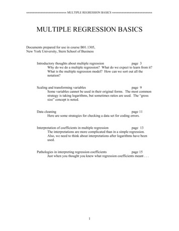
, , , , , PATHOLOGIES IN INTERPRETING REGRESSION COEFFICIENTS , , , , ,The picture below shows the locations of the points in the (G, H) plane. The values of Yare shown at some extreme points, suggesting why the apparent relationship between Yand H appears to be negative.Y 3,096Y 3,120H50Y 3,519-5727782G1787Y 3,481
0 0 0 0 0 0 0 0 REGRESSION ANALYSIS OF VARIANCE TABLE 0 0 0 0 0 0 0 0 by ygnThe quantity Syy 2imeasures variation in Y. Indeed we get sy from this asi 1sy S yyn 1. We use the symbol y i to denote the fitted value for point i. by ygnOne can show thatii 12 b y y gn b y y gn2 ii 1i2i. These sums have thei 1names SStotal, SSregression, and SSerror . They have other names or abbreviations. ForinstanceSStotal may be written as SStot .SSregression may be written as SSreg , SSfit , or SSmodel .SSerror may be written as SSerr , SSresidual , SSresid , or SSres .The degrees of freedom accounting is this:SStotalhas n - 1 degrees of freedomSSregressionhas K degrees of freedom (K is the number of independentvariables)SSerrorhas n - 1 - K degrees of freedomHere is how the quantities would be laid out in an analysis of variance table:Source ofVariationRegressionDegrees offreedomKSum of SquaresMean Squares b y y g b y y gn2 b y y gni2ii 1K b y y gniii 1n 1 KTotaln-1 by ygnii 1182MS RegressionMS Errori 1i 1n-1-K2iiErrornF2
0 0 0 0 0 0 0 0 REGRESSION ANALYSIS OF VARIANCE TABLE 0 0 0 0 0 0 0 0A measure of quality of the regression is the F statistic. Formally, this F statistic testsH 0 : β1 0, β2 0, β3 0, , βK 0 [Note that β0 does not appear.]versusH1 : at least one of β1, β2, β3, , βK is not zeroNote that β0 is not involved in this test.Also, note that sε MS Error is the estimate of σε. This has many names:standard error of estimatestandard error of regressionestimated noise standard deviationroot mean square error (RMS error)root mean square residual (RMS residual)The measure called R 2 is computed asSSRegression. This is often described as the “fractionSSTotalof the variation in Y explained by the regression.”You can show, by the way, thatsε syn 11 R2n 1 Kchn 11 R 2 is called the adjusted R-squared. This isn 1 Ksupposed to adjust the value of R2 to account for both the sample size and the number ofpredictors. With a little simple arithmetic,2 1 The quantity Radj2adjR s 1 ε sy ()219
l l l l l l l l l l l l INDICATOR VARIABLES l l l l l l l l l l l lThis document considers the use of indicator variables, also called dummy variables, aspredictors in multiple regression. Three situations will be covered.EXAMPLE 1 gives a regression in which there are independent variablestaking just two values. This is very easy.EXAMPLE 2 gives a regression in which there is a discrete independent variabletaking more than two values, but the values have a natural ordinalinterpretation. This is also easy.EXAMPLE 3 gives a regression with a discrete independent variable taking morethan two values, and these values to not correspond to an ordering. Thiscan get complicated.EXAMPLE 1Consider a regression in which the dependent variable SALARY is to be explained interms of these predictors:YEARSSKILLSSUPGENDERyears on the jobscore on skills assessment (running from 0 to 40)0 (not supervisor) or 1 (supervisor)0 (male) or 1 (female)Suppose that the fitted regression turns out to beˆSALARY 16,000 1,680 YEARS 1,845 SKILLS 3,208 SUP - 1,145 GENDERSuppose that all the coefficients are statistically significant, meaning that the p-valueslisted with their t statistics are all 0.05 or less. We have these very simple interpretations:The value associated with each year on the job is 1,680 (holding all else fixed).The value associated with each additional point on the skills assessment is 1,845(holding all else fixed).The value associated with being a supervisor is 3,208 (holding all else fixed).The value associated with being female is - 1,145 (holding all else fixed).The variables SUP and GENDER have conveniently been coded 0 and 1, and this makesthe interpretation of the coefficients very easy. Variables that have only 0 and 1 as valuesare called indicator variables or dummy variables.If the scores for such a variable are two other numbers, say 5 and 10, you mightwish to recode them.These might also be described as categorical variables with two levels.In general, we will not offer interpretations on estimated coefficients that are notstatistically significant.20
l l l l l l l l l l l l INDICATOR VARIABLES l l l l l l l l l l l lEXAMPLE 2Consider a regression in which the dependent variable HOURS (television viewing hoursper week) is to be explained in terms of predictorsINCOME (in thousands of dollars)JOB (hours per week spent at work)FAM (number of people living in the household)STRESS (self-reported level of stress, coded as1 none, 2 low, 3 some, 4 considerable, 5 extreme)The variable STRESS is clearly categorical with five levels, and we are concerned abouthow it should be handled. The important feature here is that STRESS is an ordinalcategorical variable, meaning that the (1, 2, 3, 4, 5) responses reflect the exact ordering ofstress. Accordingly, you need not take any extra action on this variable; you can use it inthe regression exactly as is.If the fitted regression equation isˆ -62.0 - 1.1 INCOME - 0.1 JOB 2.4 FAM - 0.2 STRESSHOURSthen the interpretation of the coefficient on STRESS, assuming that this coefficient isstatistically significant, is that each additional level of STRESS is associated with 0.2hour (12 minutes) less time watching television.It seems natural to encode STRESS with consecutive integers. These are some subtleties:*If you replaced the codes (1, 2, 3, 4, 5) by (-2, -1, 0, 1, 2), the regressionwould produce exactly the same estimated coefficient -0.2. Thisreplacement would alter the intercept however.*If you replaced the codes (1, 2, 3, 4, 5) by (10, 20, 30, 40, 50), theregression coefficient would be produced as -0.02.*If you do not like the equal-size spaces between the codes, you mightreplace (1, 2, 3, 4, 5) by (-3, -1, 0, 1, 3). The coefficient would nowchange from -0.2, and you’d have to rerun the regression to see what itwould be.21
l l l l l l l l l l l l INDICATOR VARIABLES l l l l l l l l l l l lEXAMPLE 3We will consider next a data set on home prices with n 370.Var
t statistics for the b’s, an F statistic for the whole regression, leverage values, path coefficients, and on and on and on and . This work is generally done by a computer program, and we’ll give