Transcription
Machine LearningBasicsLecture slides for Chapter 5 of Deep Learningwww.deeplearningbook.orgIan Goodfellow2016-09-26
TER 5. MACHINE LEARNING BASICSLinear Regression3Linear regression example0.550.502MSE(train)1yOptimization of .0w11.5Figure 5.1e 5.1: A linear regression problem, with a training set consisting of ten data pcontaining one feature. Because there is only one feature, the weight vectns only a single parameter to learn, w . (Left)Observe that linear regression l(Goodfellow 2016)
more parameters than training examples. We have little chance of chtion that generalizes well when so many wildly different solutions exxample, the quadratic model is perfectly matched to the true structsk so it generalizes well to new data.Underfitting and Overfitting inPolynomial Estimationx0OverfittingyAppropriate capacityyyUnderfittingx0x0Figure 5.25.2: We fit three models to this example training set. The training da(Goodfellow 2016)
TER 5. MACHINE LEARNING BASICSGeneralization and CapacityErrorUnderfitting zone Overfitting zoneTraining errorGeneralization errorGeneralization gap0Optimal CapacityCapacitye 5.3: Typical relationship between capacity and error. Training and testFigure5.3training error and generalizatione differently. At the left end of thegraph,(Goodfellow 2016)
Training Set SizeCHAPTER 5. MACHINE LEARNING BASICS3.5Bayes errorTrain (quadratic)Test (quadratic)Test (optimal capacity)Train (optimal capacity)Error (MSE)3.02.52.01.51.00.50.0010Figure 5.4110210310541041010Optimal capacity (polynomial degree)Number of training examples20151050010110210310Number of training examples105(Goodfellow 2016)
of how we can control a model’s tendency to overfit or underfit viacan train a high-degree polynomial regression model with differenfigure 5.5 for the results.Weight DecayAppropriate weight decay(Medium λ)x(Overfitting(λ ()yyyUnderfitting(Excessive λ)x(x(Figure5.5: We fit a high-degree polynomialregressionmodel to our example trai(Goodfellow 2016)
etween the estimator and the true value of the parameter . As is clear fquation 5.54, evaluating the MSE incorporates both the bias and the variaesirable estimators are those with small MSE and these are estimatorsanage to keep both their bias and variance somewhat in check.Bias and VarianceUnderfitting zoneBiasOverfitting citygure 5.6: As capacity increases (x-axis), bias (dotted) tends to decrease and variFigure U-shaped5.6(Goodfellow 2016)ashed) tends to increase, yielding anothercurve for generalizationerror (
0110Decision Trees010011R 5. MACHINE LEARNING 10011111001101000110101001111101110Figure 5.7 11111111110(Goodfellow 2016)
Principal Components Analysis2020101000z2x2CHAPTER 5. MACHINE LEARNING BASICS1010202020100x1102020100z11020Figure 5.8: PCA learns a linear projection that aligns the direction of greatest variancewith the axes of the new space. (Left)The original data consists of samples of x. In thisspace, the variance might occur alongdirectionsthat are not axis-aligned. (Right)TheFigure5.8transformed data z x W now varies most along the axis z1 . The direction of secondmost variance is now along z2 .(Goodfellow 2016)
Curse of DimensionalityHAPTER 5. MACHINE LEARNING BASICSFigure 5.9: As the number of relevantdimensionsFigure5.9 of the data increases (from leftight), the number of configurations of interest may grow exponentially. (Left)In tne-dimensional example, we have one variable for which we only care to distinguishegions of interest. With enough examples falling within each of these regions (each regorresponds to a cell in the illustration), learning algorithms can easily generalize correcA straightforward way to generalize is to estimate the value of the target function(Goodfellow wit2016)
Nearest NeighborFigure5.10 algorithm breaks up the inpu5.10: Illustration of how the nearestneighborgions. An example (represented here by a circle) within each region defi(Goodfellow 2016)
the manifold to vary from one point to another. This often happens whnifold intersects itself. For example, a figure eight is a manifold that has a smension in most places but two dimensions at the intersection at the centManifold 3.54.0ure 5.11: Data sampled from a distribution in a two-dimensional space that is acFigure 5.11centrated near a one-dimensional manifold,like a twisted string. The solid line indunderlying manifold that the learner should infer.(Goodfellow 2016)
Uniformly Sampled ImagesCHAPTER 5. MACHINE LEARNING BASICSFigure 5.12(Goodfellow 2016)
QMUL DatasetFigure5.13: Training examples from theQMUL5.13Multiview Face Dataset (Gong et al.ich the subjects were asked to move in such a way as to cover the two-dimenld corresponding to two angles of rotation. We would like learning algorithmo discover and disentangle such manifold coordinates. Figure 20.6 illustrates(Goodfellow 2016)
MACHINE LEARNING BASICS data significantly better than the preferred solution. For example, we can modify the training criterion for linear regression to include weight decay. To perform linear regression with weight decay, we minimize a sum . (Center)With a medium value of , the learning