WIXLIB

Multiple Logistic RegressionDr. Wan Nor ArifinUnit of Biostatistics and Research Methodology,Universiti Sains Malaysia.wnarifin@usm.my / wnarifin.pancakeapps.comWan Nor Arifin, 2015. Multiple logistic regression by Wan Nor Arifin is licensed under the Creative Commons AttributionShareAlike 4.0 International License. To view a copy of this license, visit http://creativecommons.org/licenses/by-sa/4.0/.IBM SPSS Statistics Version 22 screenshots are copyrighted to IBM Corp.4 Oct 2016Intermediate Statistics1

Outlines Introduction Steps in Multiple Logistic Regression1. Descriptive Statistics2. Variable Selection3. Model Fit Assessment4. Final Model Interpretation & Presentation4 Oct 2016Intermediate Statistics2

Objectives1.Understand the reasons behind the use of logisticregression.2.Perform multiple logistic regression in SPSS.3.Identify and interpret the relevant SPSS outputs.4.Summarize important results in a table.4 Oct 2016Intermediate Statistics3

Introduction Logistic regression is used when:– Simple logistic regression – Univariable:– Independent Variable, IV: A categorical/numerical variable.Multiple logistic regression – Multivariable:– Dependent Variable, DV: A binary categorical variable[Yes/No], [Disease/No disease] i.e the outcome.IVs: Categorical & numerical variables.Recall – Multiple Linear Regression?4 Oct 2016Intermediate Statistics4

Introduction Multiple Linear Regression– y a b1x1 b2x2 bnxnMultiple Logistic Regression–log(odds) a b1x1 b2x2 bnxn–That's why it is called “logistic” regression.4 Oct 2016Intermediate Statistics5

Introduction Binary outcome: Concerned with Odds Ratio.–Odds is a measure of chance like probability.–Odds n(Disease)/n(no Disease) among a group.–Odds Ratio, OR Odds(Factor)/Odds(No factor)–Applicable to all observational study designs.Relative Risk, RR– Only cohort study.OR RR for rare disease, useful to determine risk.4 Oct 2016Intermediate Statistics6

IntroductionFactor vs CADCADNo CADMan24 [a]76 [b]Woman(i.e. not Man)13 [c]87 [d] Odds(man) a/b 24/76 0.32 Odds(woman) c/d 13/87 0.15 OR(man/woman) 0.32/0.15 2.13 Shortcut, OR ad/bc (24x87)/(76x13) 2.114 Oct 2016Intermediate Statistics7

IntroductionFactor vs CADCADNo CADMan24 [a]76 [b]Woman(i.e. not Man)13 [c]87 [d] Risk(man) Proportion CAD a/(a b) 0.24 Risk(woman) Proportion CAD c/(c d) 0.13 RR(man/woman) 0.24/0.13 1.85 OR, 2.114 Oct 2016Intermediate Statistics8

Steps in Multiple Logistic Regression Dataset: slog.sav Sample size, n 200 DV: cad (1: Yes, 0: No) IVs:–Numerical: sbp (systolic blood pressure), dbp (diastolicblood pressure), chol (serum cholesterol in mmol/L), age(age in years), bmi (Body Mass Index).–Categorical: race (0: Malay, 1: Chinese, 2: Indian), gender (0:Female, 1: Male)4 Oct 2016Intermediate Statistics9

Steps in Multiple Logistic Regression1.Descriptive statistics.2.Variable selection.a. Univariable analysis.b. Multivariable analysis.c. Multicollinearity.d. Interactions.3.Model fit assessment.4.Final model interpretation & presentation.4 Oct 2016Intermediate Statistics10

1. Descriptive statistics Set outputs by CADstatus.–Data Split File Select Compare groups–Set Groups Based on:cad, OK4 Oct 2016Intermediate Statistics11

1. Descriptive statistics Obtain mean(SD) andn(%) by CAD group.–Analyze DescriptiveStatistics Frequencies–Include relevantvariables in Variables4 Oct 2016Intermediate Statistics12

1. Descriptive statistics Cont.–Statistics tick Continue4 Oct 2016Intermediate Statistics13

1. Descriptive statistics Cont.–Charts tick Continue OK4 Oct 2016Intermediate Statistics14

1. Descriptive statistics Results4 Oct 2016Intermediate Statistics15

1. Descriptive statistics Results4 Oct 2016Intermediate Statistics16

1. Descriptive statistics Results– Look at histograms todecide data normality fornumerical variables.Remember your Basic Stats!Caution! Reset back thedata.–Data Split File SelectAnalyze all cases–OK4 Oct 2016Intermediate Statistics17

1. Descriptive statistics Present the results in a table.FactorsCAD, n 37mean(SD)No CAD, n 163mean(SD)Systolic Blood Pressure143.8(25.61)129.3(22.26)Diastolic Blood 4(64.9%)13(35.1%)76(46.6%)87(53.4%)4 Oct 2016Intermediate Statistics18

2. Variable selection To select best variables to predict the outcome. Sub-steps:a. Univariable analysis.b. Multivariable analysis.c. Checking multicollinearity & interactions.4 Oct 2016Intermediate Statistics19

2a. Univariable analysis Perform Simple Logistic Regression on each IV. Select IVs which fullfill:–P-value 0.25 Statistical significance.–Clinically significant IVs You decide.4 Oct 2016Intermediate Statistics20

2a. Univariable analysis Analyze numericalvariables:–Analyze Regression Binary Logistic–Dependent: cad,Covariates: sbp–Click Options TickIteration history, CI forexp(B) Continue OK–Repeat for dbp, chol, age,bmi4 Oct 2016Intermediate Statistics21

2a. Univariable analysis ResultsModel: SBP Pvalue 0.001 byLikelihood Ratio (LR)test SBP P-value 0.001 byWald test 4 Oct 2016Intermediate StatisticsExp(B) is OR.OR(1 unit in SBP) 1.04(95% CI: 1.01,1.04). Unadjusted/Crude OR.Interpretation:1mmHg increase inSBP increase odds ofCAD by 1.02 times.In variable selectioncontext, less concernabout OR &interpretation.22

2a. Univariable analysis Analyze categoricalvariables:–Dependent: cad,Covariates: gender–Click Categorical Categorical Covariates:gender Change Contrast Reference Category:First Change Continue.–Repeat for race4 Oct 2016Intermediate Statistics23

2a. Univariable analysis ResultsWomen 0 becomesthe reference group. Model: Gender Pvalue 0.044 by LR test Gender P-value 0.048by Wald test4 Oct 2016Intermediate StatisticsOR(male) 2.11(95%CI: 1.01, 4.44).Unadjusted/CrudeOR.Interpretation: Manhas 2.11 times oddsof CAD as comparedto woman.24

2a. Univariable analysis P-values of IVs – select P-value 0.25FactorsP-value (Wald test)P-value (LR test)Systolic Blood Pressure0.0010.001Diastolic Blood 0.8870.8520.981*GenderMan- Woman0.0480.044*For both variables4 Oct 2016Intermediate Statistics25

2b. Multivariable analysis Selected variables:– sbp, dbp, chol, age, genderPerform Multiple logistic regression of the selectedvariables (multivariable) in on go.Variable selection is now proceed at multivariablelevel.Some may remain significant, some becomeinsignificant.4 Oct 2016Intermediate Statistics26

2b. Multivariable analysis Variable SelectionMethods:–Automatic. –Forward: Conditional, LR,Wald. Enters variables.Backward: Conditional, LR,Wald. Removes variables.Manual. 4 Oct 2016Enter. Entry & removal ofvariables done manually.(Recommended, but leave toexperts/statisticians).Intermediate Statistics27

2b. Multivariable analysis Variable Selection in this workshop:–Automatic by Forward & Backward LR.–Selection of variables by P-values based on LR test.4 Oct 2016Intermediate Statistics28

2b. Multivariable analysis Enter all selected variables. Perform 2x – 1x Forward LR, 1x Backward LR.Options: Just leave at the default values.4 Oct 2016Intermediate Statistics29

2b. Multivariable analysis ResultsForward LR Both methodskeep sameIVs: dbp &gender.P-values byWald test.Backward LR4 Oct 2016Intermediate Statistics30

2b. Multivariable analysis ResultsForward LR Both methods keep sameIVs: dbp & gender.P-values by LR test.Backward LR4 Oct 2016Intermediate Statistics31

2c. Multicollinearity Indicates redundant variables –highly correlated IVs.Perform Enter method with dbp &gender.Look at coefficients (B) & stderrors (SE) / ORs (95% CIs) if theyare suspiciously large.Results 4 Oct 2016Intermediate StatisticsSEs are quite smallrelative to Bs.95% CIs are not toowide.No multicollinearity.32

2d. Interactions IVs combination thatrequires interpretation ofregression separately basedon levels of IV makingthings complicated.Perform Enter method withdbp, gender & dbp x gender.Select both dbp & gender(hold Ctrl on keyboard) Click a*b 4 Oct 2016Intermediate Statistics33

2d. Interactions ResultsWald test for dbp by gender(dbp*gender) not sig. Canremove the interaction termfrom model.4 Oct 2016Intermediate Statistics34

2. Variable selection At the end of Variable Selection Step PreliminaryFinal Model. P-values by Waldtest per variableby Enter method.Take this adjustedOR.P-values by LR test forboth dbp & gender byEnter method.P-values by LR pervariable. Obtained withForward LR method.4 Oct 2016Intermediate Statistics35

3. Model fit assessment By these 3 goodness-of-fit assessment methods:a. Hosmer-Lemeshow testb. Classification table.c. Area under Receiver Operating Characteristics (ROC)curve. At the end Final Model.4 Oct 2016Intermediate Statistics36

3. Model fit assessment Perform Enter method withdbp & gender.Additionally–Click Options. TickHosmer-Lemeshowgoodness-of-fit–Click Save TickProbabilities underPredicted Values–A new variable PRE 1 will becreated.4 Oct 2016Intermediate Statistics37

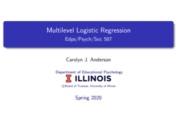
3a. Hosmer-Lemeshow test Indicates fit of Preliminary Final Model to data. ResultsP-value 0.09 0.05 Good model fit to the data.Observed counts in data. 4 Oct 2016Intermediate StatisticsExpected/predicted countsby model.The smaller the differencesbetween Observed vsExpected Better model fitto data.38

3b. Classification table CAD & No CAD subjects observed vspredicted/classified by Preliminary Final Model.% correctly classified 70% is expected for goodmodel fit.Results 4 Oct 2016Intermediate Statistics80% of subjects arecorrectly classified bythe model.Good model fit to thedata.39

3c. Area under ROC curve (AUC) A measure of ability of the model todiscriminate CAD vs Non CADsubjects.AUC 0.7 is acceptable fit.AUC 0.5 no discrimination at all,not acceptable.Steps–Analyze ROC curve. Assign TestVariable: Predicted probability (PRE 1),State Variable: cad, Value of StateVariable: 1.–Under Display tick ROC Curve, Withdiagonal reference line and StandardError and confidence interval.4 Oct 2016Intermediate Statistics40

3c. Area under ROC curve (AUC) Results 4 Oct 2016AUC 0.73 0.7.95% CI: 0.64, 0.82.Lower limit slightly 0.7, stillacceptable 0.5.Good model fit to the data.Intermediate Statistics41

3. Model fit assessment All 3 methods indicate good model fit ofPreliminary Final Model.Can conclude the model with dbp & gender FinalModel.4 Oct 2016Intermediate Statistics42

2. Final Model interpretation & presentation The Final Model. P-values by Waldtest per variableby Enter method.Take this adjustedOR.P-values by LR test forboth dbp & gender byEnter method.P-values by LR pervariable. Obtained withForward LR method.4 Oct 2016Intermediate Statistics43

4. Final Model interpretation & presentation Associated factors of coronary artery disease.aFactorsbAdjusted OR (95% CI)P-valueaDiastolic Blood Pressure0.051.05 (1.02, 1.08) 0.001Gender0.812.24 (1.04, 4.82)0.036Man vs WomanLR test1mmHg increase in DBPincrease odds of CADby 1.05 times, whilecontrolling for gender.Man has 2.24 times odds ofCAD as compared to woman,while controlling for DBP.To obtain for 10mmHg increase in DBPOR exp(c x b) exp(10 x 0.05) exp(0.5) 1.65 times.4 Oct 2016Intermediate Statistics44

Q&A4 Oct 2016Intermediate Statistics45

2.Perform multiple logistic regression in SPSS. 3.Identify and interpret the relevant SPSS outputs. 4.Summarize important results in a