WIXLIB

Simple Linear and Multiple RegressionIn this tutorial, we will be covering the basics of linear regression, doing both simple andmultiple regression models. The following data gives us the selling price, squarefootage, number of bedrooms, and age of house (in years) that have sold in aneighborhood in the past six 00155500165000Square Age30253040183019710133102103We need to develop three simple regression models to predict the selling price basedon each of the individual factors and determine which one is the best model. Next, wewill develop a model to predict the selling price of a house based on the square footage,number of bedrooms, and age and will discuss if all three variables should be includedand if it is a better model than just the three simple regression models.

To use Excel for regression, we do not want to use the Excel QM module, but rather willbe using the data analysis add-in. To check and be sure that it is activated, go to File Options Add-ins. An Excel Options window will appear as shown here.

Under Active Application Add-ins be sure that Analysis ToolPak is there.

If not, click the “Go” button at the bottom of the window next to “Manage Excel Add-Ins”and simply tick the box next to Analysis ToolPak and Analysis ToolPak VBA thenclick OK.Once you have the Add-ins in place, you are ready to get started.

1. Enter or copy the data from the table above into a blank Excel spreadsheet as shownhere.

2. Click on Data Data Analysis and, in the Data Analysis pop-up window, scroll downand select Regression and click OK.3. Click in the box for Input Y Range and this is going to be our dependent variable, orin this case, the selling price, so highlight cells A3-A20.

4. Our first independent variable will be square footage, so click in the box for Input XRange and select cells B3-B20. Be sure that the box is ticked next to Labels and selectthe Output Range as F3.5. Click OK. This will put the regression output next to our data table.

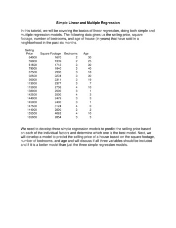
Repeat steps 2-5, but select C3-C20 for the number of bedrooms and put the OutputRange as F23, then, repeat steps 2-5 again but select D3-D20 for Age, and put theOutput Range as F43.You should now have all three simple regression models. Click here to download thecompleted sample spreadsheet so you can compare it to yours.The key parts of this output are as follows (using the square footage example):Under the “Regression Statistics” Multiple R – the correlation coefficient – notes the strength of the relationship – inthis case, 0.80358 – a pretty strong positive relationship. R squared – the amount of variability in the dependent variable explained by theindependent variable(s). In this case, 0.6457 – again, a pretty strong number –almost 65% of the variability in purchase price is explained by square footage. Adjusted R squared – this is when you have more than one independent variableand have adjusted the R squared value for the number of independent variables.Use this when looking at a multiple regression model.Under the ANOVA Tables Significance F – this tests the significance of the overall model. We look for thisto be less than 0.05. If it is less than 0.05, we can reject the null hypothesis anddetermine that the model is statistically valid. In this case, it’s 0.000102, so wehave a valid model. Intercept Coefficient – this is the intercept for our line if we were to plot it out.With X as zero, this is where the line crosses the Y axis. Here its 2367. So ahouse with zero square feet will sell for 2,367. X Coefficient – this is the coefficient for our independent variable for the linearequation. It is the slope of our line or the amount that our dependent variablechanges for every 1 change in our independent variable. For every increase insquare footage by one, our price will change by this amount, or 46.6. X P-Value – this tests the significance of the variable. We look for this to be lessthan 0.05. If it less than 0.05, we can reject the null hypothesis and determinethat the variable is statistically significant. It’s 0.000102, so we have a significantvariable.

Running a multiple regression is the same as a simple regression, the only differencebeing that we will select all three independent variables as our ‘X variables’ – our InputY Range is A3-A20 while our Input X Range is now B3-D20. Again, be sure to tick thebox for Labels and this time select New Worksheet Ply as your Output option.Click here to download the completed sample spreadsheet so you can compare it toyours.If we look at those statistics for all three simple models and our multiple regressionmodel, we get the following:ModelSquareFootageBedroomsAgeMultiple model:SFBedroomsAgeSignificanceMultiple usted 59861.604196.881338.941348Comparing the three simple models, we can see that the model using age as thepredictor of price is the best. It has the highest Multiple R (i.e., strongest relationship)and highest R-Square (explains most of the variability in the dependent variable).

Looking at the multiple model, this is even better. Both Multiple R and R-Square arehigher, even when adjusting for the number of dependent variables. What is interestinghere is that the number of bedrooms is not significant in this model, so that should notbe included in the final model.This concludes the tutorial on both simple and multiple regression models.

To use Excel for regression, we do not want to use the Excel QM module, but rather will be using the data analysis add-in. To check and be sure that it is activated, go to File Options Add-ins. An Excel Options window will appear as shown here. Under Active Application Add-ins be sure that Analysis ToolPak is there. If not, click the “Go” button at the bottom of the window next to .