WIXLIB

Practical Guide to theSimplex Method of Linear ProgrammingMarcel OliverRevised: September 28, 20201The basic steps of the simplex algorithmStep 1: Write the linear programming problem in standardformLinear programming (the name is historical, a more descriptive term wouldbe linear optimization) refers to the problem of optimizing a linear objectivefunction of several variables subject to a set of linear equality or inequalityconstraints.Every linear programming problem can be written in the following standard form.Minimize ζ cT x(1a)Ax b ,(1b)x 0.(1c)subject toHere x Rn is a vector of n unknowns, A M (m n) with n typicallymuch larger than m, c Rn the coefficient vector of the objective function,and the expression x 0 signifies xi 0 for i 1, . . . , n. For simplicity, weassume that rank A m, i.e., that the rows of A are linearly independent.Turning a problem into standard form involves the following steps.(i) Turn Maximization into minimization and write inequalities in standard order.This step is obvious. Multiply expressions, where appropriate, by 1.1

(ii) Introduce slack variables to turn inequality constraints into equalityconstraints with nonnegative unknowns.Any inequality of the form a1 x1 · · · an xn c can be replaced bya1 x1 · · · an xn s c with s 0.(iii) Replace variables which are not sign-constrained by differences.Any real number x can be written as the difference of nonnegativenumbers x u v with u, v 0.Consider the following example.Maximize z x1 2 x2 3 x3(2a)x1 x2 x3 1 ,(2b) 2 x1 x2 2 x3 5 ,(2c)x1 x2 4 ,(2d)x2 x3 5 ,(2e)x1 0 ,(2f)x2 0 .(2g)subject toWritten in standard form, the problem becomesminimize ζ x1 2 x2 3 u 3 v(3a)x1 x2 u v 1 ,(3b)2 x1 x2 2 u 2 v s 1 5 ,(3c)x1 x2 s 2 4 ,(3d)x2 u v s 3 5 ,(3e)x1 , x2 , u, v, s1 , s2 , s3 0 .(3f)subject toStep 2: Write the coefficients of the problem into a simplextableauThe coefficients of the linear system are collected in an augmented matrixas known from Gaussian elimination for systems of linear equations; thecoefficients of the objective function are written in a separate bottom rowwith a zero in the right hand column.For our example, the initial tableau reads:2

x11210 1x21 1 11 2u 1 201 3v120 13s101000s200100s30001015450In the following steps, the variables will be divided into m basic variablesand n m non-basic variables. We will act on the tableau by the rules ofGaussian elimination, where the pivots are always chosen from the columnscorresponding to the basic variables.Before proceeding, we need to choose an initial set of basic variableswhich corresponds to a point in the feasible region of the linear programming problem. Such a choice may be non-obvious, but we shall defer thisdiscussion for now. In our example, x1 and s1 , . . . , s3 shall be chosen as theinitial basic variables, indicated by gray columns in the tableau above.Step 3: Gaussian eliminationFor a given set of basic variables, we use Gaussian elimination to reducethe corresponding columns to a permutation of the identity matrix. Thisamounts to solving Ax b in such a way that the values of the nonbasicvariables are zero and the values for the basic variables are explicitly givenby the entries in the right hand column of the fully reduced matrix. Inaddition, we eliminate the coefficients of the objective function below eachpivot.Our initial tableau is thus reduced tox110000x21 3 21 1u 1011 4v10 1 14s101000s200100s30001013351The solution expressed by the tableau is only admissible if all basic variablesare non-negative, i.e., if the right hand column of the reduced tableau is freeof negative entries. This is the case in this example. At the initial stage,however, negative entries may come up; this indicates that different initialbasic variables should have been chosen. At later stages in the process, the3

selection rules for the basic variables will guarantee that an initially feasibletableau will remain feasible throughout the process.Step 4: Choose new basic variablesIf, at this stage, the objective function row has at least one negative entry,the cost can be lowered by making the corresponding variable basic. Thisnew basic variable is called the entering variable. Correspondingly, oneformerly basic variable has then to become nonbasic, this variable is calledthe leaving variable. We use the following standard selection rules.(i) The entering variable shall correspond to the column which has themost negative entry in the cost function row. If all cost functioncoefficients are non-negative, the cost cannot be lowered and we havereached an optimum. The algorithm then terminates.(ii) Once the entering variable is determined, the leaving variable shall bechosen as follows. Compute for each row the ratio of its right handcoefficient to the corresponding coefficient in the entering variable column. Select the row with the smallest finite positive ratio. The leavingvariable is then determined by the column which currently owns thepivot in this row. If all coefficients in the entering variable columnare non-positive, the cost can be lowered indefinitely, i.e., the linearprogramming problem does not have a finite solution. The algorithmthen also terminates.If entering and leaving variable can be found, go to Step 3 and iterate.Note that choosing the most negative coefficient in rule (i) is only aheuristic for choosing a direction of fast decrease of the objective function.Rule (ii) ensures that the new set of basic variables remains feasible.Let us see how this applies to our problem. The previous tableau holdsthe most negative cost function coefficient in column 3, thus u shall be theentering variable (marked in boldface). The smallest positive ratio of righthand column to entering variable column is in row 3, as 13 51 . The pivotin this row points to s2 as the leaving variable. Thus, after going throughthe Gaussian elimination once more, we arrive at4

x110000x2 1 3 23 9u00100v00 100s101000s2101 14s300010433213At this point, the new entering variable is x2 corresponding to the onlynegative entry in the last row, the leaving variable is s3 . After Gaussianelimination, we findx110000x200010u00100v00 100s101000s2s32313 11513231313323319 311143Since there is no more negative entry in the last row, the cost cannot be lowered by choosing a different set of basic variables; the termination conditionapplies.Step 4: Read off the solutionThe solution represented by the final tableau has all nonbasic variables set tozero, while the values for the basic variables can be can be read off the righthand column. The bottom right corner gives the negative of the objectivefunction.213In our example, the solution reads x1 143 , x2 3 , x3 u 3 , s1 5,v s2 s3 0, which corresponds to ζ 19, which can be independentlychecked by plugging the solution back into the objective function.As a further check, we note that the solution must satisfy (2b), (2d),and (2e) with equality and (2c) with a slack of 5. This can also be checkedby direct computation.2InitializationFor some problem it is not obvious which set of variables form a feasibleinitial set of basic variables. For large problems, a trial-and-error approach5

nis prohibitively expensive due the rapid growth of m, the number of possibilities to choose m basic variables out of a total of n variables, as m and nbecome large. This problem can be overcome by adding a set of m artificialvariables which form a trivial set of basic variables and which are penalizedby a large coefficients ω in the objective function. This penalty will causethe artificial variables to become nonbasic as the algorithm proceeds.We explain the method by example. For the problemminimize z x1 2 x2 2 x3(4a)x1 x2 2 x3 x4 5 ,(4b)x1 x2 x3 x4 5 ,(4c)x1 2 x2 2 x3 x4 6 ,(4d)x 0,(4e)subject towe set up a simplex tableau with three artificial variables which are 2122x41 1 105560We proceed as before by first eliminating the nonzero entries below thepivots:a11000a20100a30010x11111 3ωx21122 4ωx32122 5ωx41 1 1ω556 16ωSince, for ω large, 2 5ω is the most negative coefficient in the objectivefunction row, x3 will be entering and, since 52 62 51 , a1 will be leaving.The Gaussian elimination step then yields6

a1a2010012 12 1 1 52 ωa30010x1x2121212120 12 ω11 32 ωx31000x412 32 2 1 72 ω52521 5 72 ωNow x2 is entering, a3 is leaving, and we obtaina110 1ωa20100a3 12 121 1 23 ωx1x2001012120 12 ωx31000x432 12 21 12 ω221 6 2ωThe new entering variable is x1 while the criterion for the leaving variableis tied between a2 and x3 . Since we want the artificial variable to becomenonbasic, we take a2 to be leaving. (Choosing x3 as the leaving variablewould lead us to the same solution, albeit after a few extra steps.) Weobtaina110 1ωa2 120ωa30 11 1 ωx10100x20010x31000x42 1 21041 6The termination condition is now satisfied, and we see that the solution isz 6 with x1 4, x2 1, x3 0, x4 0.We close with two remarks. When using a computer to perform the simplex algorithm numerically,ω should be chosen large (one or two orders of magnitude larger thanany of the other coefficients in the problem) but not too large (to avoidloss of significant digits in floating point arithmetic). If not all artificial variables become nonbasic, ω must be increased. Ifthis happens for any value of ω, the feasible region is empty. In the final tableau, the penalty parameter ω can only appear in artificial variable columns.7

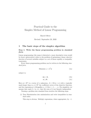
3DualityThe concept of duality is best motivated by an example. Consider thefollowing transportation problem. Some good is available at location A atno cost and may be transported to locations B, C, and D according to thefollowing directed graph:4 B14A2*! D3 5COn each of the unidirectional channels, the unit cost of transportation is cjfor j 1, . . . , 5. At each of the vertices bα units of the good are sold, whereα B, C, D. How can the transport be done most efficiently?A first, and arguably most obvious way of quantifying efficiency would beto state the question as a minimization problem for the total cost of transportation. If xj denotes the amount of good transported through channel j,we arrive at the following linear programming problem:minimize c1 x1 · · · c5 x5(5a)x1 x3 x4 bB ,(5b)x2 x3 x5 bC ,(5c)x4 x5 bD .(5d)subject toThe three equality constraints state that nothing gets lost at nodes B, C,and D except what is sold.There is, however, a second, seemingly equivalent way of characterizingefficiency of transportation. Instead of looking at minimizing the cost oftransportation, we seek to maximize the income from selling the good. Letting yα denote the unit price of the good at node α A, . . . , D with yA 0by assumption, the associated linear programming problem is the following:maximize yB bB yC bC yD bD8(6a)