Transcription
Finite Element Modeling of Deformation Behavior of Steel Specimens underVarious Loading ScenariosDilip Banerjee1,a*, Mark Iadicola1,b, Adam Creuziger1,c, and Timothy Foecke1,d1Material Measurement Laboratory, NIST, 100 Bureau Dr, Gaithersburg, MD 20899, USAaDilip.Banerjee@nist.gov, bMark.Iadicola@nist.gov, eywords: uniaxial and biaxial tensile tests, finite element modeling, steel, cruciformAbstract. Lightweighting materials (e.g., advanced high strength steels, aluminum alloys etc.) areincreasingly being used by automotive companies as sheet metal components. However, accuratematerial models are needed for wider adoption. These constitutive material data are often developedby applying biaxial strain paths with cross-shaped (cruciform) specimens. Optimizing the design ofspecimens is a major goal in which finite element (FE) analysis can play a major role. However,verification of FE models is necessary. Calibrating models against uniaxial tensile tests is a logicalfirst step. In the present study, reliable stress-strain data up to failure are developed by using digitalimage correlation (DIC) technique for strain measurement and X-ray techniques and/or force datafor stress measurement. Such data are used to model the deformation behavior in uniaxial andbiaxial tensile specimens. Model predictions of strains and displacements are compared withexperimental data. The role of imperfections on necking behavior in FE modeling results of uniaxialtests is discussed. Computed results of deformation, strain profile, and von Mises plastic strain agreewith measured values along critical paths in the cruciform specimens. Such a calibrated FE modelcan be used to obtain an optimum cruciform specimen design.1. IntroductionAutomotive companies are actively interested in the increased use of advanced lightweightingmaterials such as advanced high strength steels (AHSS), aluminum alloys etc. as sheet metalcomponents. However, accurate material models are needed before these materials can be widelyused. These material models are often developed using linear strain paths using cross-shaped biaxialspecimens (i.e., cruciform) [1, 2, 3]. But successful cruciform mechanical testing is dependent onthe specimen design itself. In the past, a wide variety of designs have been used [4, 5, 6, 7]. Thespecimen design should meet certain goals: (a) Both strain uniformity and eventual failure in thebiaxially loaded gauge area, (b) reduction of stress concentration outside of the gauge area, (c)minimization of shear strains in the gauge area, and (d) similar behavior during repeat tests. Aprudent approach for obtaining optimum specimen design is to combine FE simulation withoptimization software such that the above objectives are achieved. But the first step is to calibratethe FE model against precise experimental measurements. These measurements were obtained usingthe state of the art mechanical testing facility at the National Institute of Standards and Technology(NIST) Center for Automotive Lightweighting (NCAL) [8]. In this paper, the verification of FEmodels against experimental measurements is discussed for both uniaxial and biaxial tensile tests.Additionally, plastic deformation behavior in the specimens is discussed. Note that uncertaintiesassociated with the measurement of displacement and strain are reported in ref [9].2. Uniaxial Tensile Tests2.1 Uniaxial Tensile Test Experiments. Uniaxial test specimens were made of two different steels:(a) 9.525 mm (0.375 in) thick hot-rolled low carbon steel (hereinafter called “thick specimen”) and(b) 3.038 mm (0.1196 in) thick cold-rolled AISI 1008 steel (hereinafter called “thin specimen”).This thin specimen steel has much lower yield and ultimate tensile strength than the thick specimen
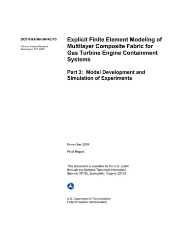
Force, kNTrue stress, MPasteel. Uniaxial tests were conducted both to verify the FE model and to generate stress-strain datafor uniaxial and biaxial tensile tests. Uniaxial tensile tests were performed for both steels in therolling direction of the sheet. These tests were performed using the X-axis of the cruciformmachine and the DIC system [8]. The gauge section as designed has a nominally parallel length of101.6 mm and width of 19.05 mm with radii of 50.8 mm to the 28.58 mm wide end-tabs. The sameplanar geometry was used for both thicknesses of material. Since the biaxial test and model willachieve strains beyond the uniform strain of a900standard tensile test, it was necessary to800700approximate the true-stress/true-straina600relationship at strains beyond uniformb500deformation. The true axial strain was400calculated as the average strain across the3009.525 mm (0.375 in) (thick) specimen200width for each point in time in the axial3.175 mm (0.125 in) (thin) specimen100direction at the eventual location of failure.0The true stress was calculated as the applied00.511.5force divided by the current cross-sectionalTrue strainarea at the same location and time. TheFig. 1. True stress – true strain data obtained inresulting stress strain curves are shown inuniaxial tensile tests.Fig. 1. The uniaxial test for the thin materialused a constant displacement rate, which resulted in an undesirable increase in strain rate fromapproximately 8x10⁻⁵ s-1 before initial localization (maximum force) to 2x10⁻³ s-1 as the sampleapproached failure. In the thick material uniaxial test the displacement rate was reduced twiceduring the test (at approximately 0.26 and 0.49 true strain) to keep the average strain ratenear 9x10⁻⁴ s-1. Following the tensile tests, history-dependent axial displacement values at locationsin the end-tabs approximately 82 mm away from the central point were extracted for subsequent usein the FE simulation as boundary conditions (BC). The displacement values were interpolated fromthe DIC field data at the FE nodal coordinate values nearest to X 82 mm along the axial direction.The force-displacement curve for the thick specimen is shown in Fig. 2. Displacement andstrain data corresponding to the four loading points (A, B, C, and D) in Fig. 2 were extracted forcomparison with FE results. Such axial100displacement vs. x-coordinate data as measured80Cby the DIC system were output along threeBA60specimen lines (i.e., along centerline, alongDlines 4.63 mm away from centerline) in the40axial direction. Only centerline data are used in20this study.Comparison points001020Displacement, mmFig. 2. Force-displacement curves for the thickspecimen.1302.2 FE Simulation of Uniaxial Tensile Tests.A 3D finite element model of the thick uniaxialspecimen was developed using ABAQUS1software [10]. Constitutive material model datawere obtained from experimental stress-strainCertain commercial software or materials are identified to describe a procedure or concept adequately. Suchidentification is not intended to imply recommendation, endorsement, or implication by NIST that the software ormaterials are necessarily the best available for the purpose.
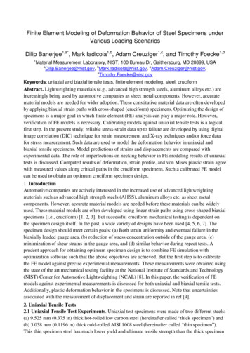
data in uniaxial tension tests (Fig. 1). Isotropic hardening is assumed in this study. Young’smodulus of 210 GPa and Poisson ratio of 0.3 were assumed for both materials. A 1/2 symmetry FEmodel was developed by taking advantage of the mirrorsymmetry in the specimen shape and loading. The solidmodel was developed using mapped meshing, and 3D linearNodeshifthexahedral elements (C3D8R) were used. Fig. 3 shows atypical FE mesh. In order to introduce instability in thesimulation, geometric imperfections were introduced. Thiswas accomplished by physically displacing nodes at theedge by a small fraction of the grid spacing (see Fig. 3).Note that all the nodes through the depth at this edgelocation were displaced by the same amount. This is similarto the concept of creating a notch to initiate instability.ABAQUS simulations showed that the ultimate failureFig. 3. Finite element mesh and aoccurred near the vicinity of this imperfection but not at theschematic showing node shift usedexact point of imperfection. Experiments on the thickto introduce instability in FEspecimens showed the formation of Lüders bands (typicallysimulation.encountered in low carbon steels). The eventual necking and failure occurred near the locationswhere Lüders bands initiated. Therefore, it was necessary to capture this behavior in the FEsimulation by introducing imperfections near the regions where the Lüders bands were seen.Figure 4 shows both the measured and computed axial displacements along the centerline of thespecimen for points corresponding D in Fig. 2. Good agreement was seen except for the point nearthe necking region. This is because there is a slight difference between the model predicted locationof necking and that obtained in the experiment. Additionally, the model seems to predict a sharperlocalization than that seen in the experimental results. Figure 5 shows the comparison between themeasured von Mises equivalent strain and computed von Mises plastic strain plots. Again, theagreement is good in terms of the overall shape and maximum values. However, ABAQUS valuesslightly under-predict the strains away from the maximum localization point. This isunderstandable, as ABAQUS plots do not include the elastic component of the strain (which is quitesmall compared to the plastic component of the strain). Figure 6 shows measured and computedcontour plots of von Mises equivalent strain on the surface of the specimen. The overall strainprofile along the specimen length as computed by ABAQUS agrees well with measured values.1.4von Mises equivalent strainCenterline (D)Longitudinal displacement, ance along specimen length, mmFig. 4. Measured and computed longitudinaldisplacements along the specimen lengthcorresponding to the point D in Fig. 2.1.210.8ExperimentABAQUS0.60.40.2-500-0.2 050100100Distance along specimen length, mmFig. 5. von Mises equivalent strain and ABAQUScomputed von Mises plastic strain along thespecimen length corresponding to point D in Fig. 2.
DIC MeasurementsABAQUS computed plotFig. 6. Contour plots of measured von Mises equivalent strain and ABAQUS computedvon Mises plastic strain along the specimen length corresponding to point D in Fig. 2.3. Biaxial Tensile Tests3.1 Cruciform Specimen Design. Cruciform geometries for in-plane biaxial tests are advantageousbecause (a) the region of interest is far away from locations where BCs are applied and (b) varyingstrain ratios can be applied along the arms of the specimen. In most of the specimen designs, failureoccurred outside the central gauge section of interest and at strains well below traditional forminglimit strains, due to a combination of various factors such as stress and deformation concentrationsat corners or near slits in the arms [11]. In some designs, the central gauge section is thinned downto achieve higher strain and possibly failure in the middle of the gauge section. In this study, thespecimen design follows that of ref. [7], with the initial specimen being enlarged in all threedirections to a thickness of 0.953 mm. The present specimen design for the thick specimen isdescribed in ref [9]. Cruciform samples were machined by water-jet with the X-axis aligned withthe rolling direction of the sheet. A similar geometry was used for the thin specimen, except that ithad a designed thickness of 0.749 mm (0.0295 in) in the thinned down region in the center and thatthe fillet radius at the peripheral region of the central pocket was 0.397 mm (0.016 in).3.2 Biaxial Tensile Tests. Biaxial loading was applied using four hydraulic actuators, which arecontrolled in orthogonal pairs [11]. Each of these actuators has 500 kN load capacity and has a 50mm displacement range from a reference distance of 640 mm between grip faces on the X or Y-axis.Details of the loading and in situ DIC data acquisition are described in [11]. In the present study, thebiaxial tests were conducted using displacement control. Fig. 7 shows force-displacement curves.The 3D displacement of top surface about the center of the cruciform specimen was measured witha stereo DIC system. Surface strains are calculated from the measured displacement fields.Measured, history-dependent average U and V values at locations approximately 25 mm away fromthe central point were extracted for subsequent use in FE simulation (see Fig. 8). Since cruciformspecimens tend to concentrate strain in the corners between the arms leading to premature failure, itis important for FE model to be able to capture the mechanical behavior in these corners.Accordingly, measured displacement and strain data were extracted along a diagonal line thatbisects the region between the central pocket and the reentrant radius at the meeting point of the Xand Y arms (see "Path" in Fig. 8). These data are compared to FE data corresponding to loadingpoints shown in Fig. 7. Results are shown here for only the maximum force point in Fig. 7.3.3 FE Modeling. A 3D FE model of the cruciform specimens was developed using ABAQUSsoftware [10]. See section 2.2 for details on material data. A 1/8th symmetry model was developed
752060Force, kN2515451030Displacement boundaryconditionPath5thin materialcomparison points"thick material"15Fig. 8. A portion of the FE mesh of the thincruciform specimen along with locations for axial00displacement boundary conditions. Also shown is0246Displacement, mmthe path on which the FEA results are extractedFig. 7. Force-displacement curves for X-axis from for comparison with experimental measurements.cruciform specimens.by using the mirror symmetry in the specimen shape and loading. FE model included both regular(C3D8) and reduced integration brick (C3D8R) elements. In addition to symmetry conditions, axialdisplacement boundary conditions were applied on each arm (Fig. 8). Simulated results wereextracted for all points labeled in Fig. 7 along the path shown in Fig. 8 and compared with DIC data.Only data corresponding to the maximum force point are discussed below for the thin specimen.3.4 Results and Discussion. Fig. 9 shows bothU-expt-1experimental and computed U displacement fields. ThereU-expt-40.8are four equivalent paths for which experimental dataU-expt-3U-expt-2have been measured. However, because of the symmetry0.6ABAQUS-U-C3D8Rused in the model, only one plot is available for the FE0.4ABAQUS-U-C3D8model. Two sets of ABAQUS results are shown (one0.2each for C3D8R and C3D8 element). Fig. 9 shows thata0the model predicts the displacement field correctly. Fig.010203010 shows plots of normal strains in the Z direction. The-0.2Distance along path, mmmeasured thickness strains were calculated assumingFig. 9. U displacement along path involume conservation, using ezz -(exx eyy). ABAQUSFig.8: U-expt-1 etc. (measured);simulations with C3D8 elements are in better agreementABAQUS-U-C3D8 etc. (computed).with experimental results. However, the modeled peakezz for C3D8 element exceeds those seen in experimental data. It is also noticed that the modelpredicts a slightly narrower width of the ezz profile than that in the experimental results. Themeasured von Mises equivalent strain plot is shown in Fig. 11. This plot is compared with the vonMises equivalent plastic strain (PEEQ) in ABAQUS. This comparison is justified since elastic strainis very small. Fig. 11 shows the largest value at the reentrant radius of about 0.38 and around 0.084in the central region. Uniform equivalent strain is seen in the central pocket, which is also seen inthe ABAQUS results in Fig. 12. The ABAQUS results show a value of 0.16 in the central pocketand a value of 0.3 at the outer edge of the reentrant corner. The model shows a slight decrease instrain along the diagonal from the reentrant radius to the peripheral region of the central pocket,where a value of about of 0.24 is obtained. Although the model does not show as thick a band ofPEEQ of 0.3 along the diagonal from the reentrant radius to the peripheral region of the centralpocket (as seen in experimental result in Fig. 11), it is intuitive that the failure initiation willprobably start at the strain concentration at the base of the fillet from the thicker region into thethinner region. In fact, the experiment showed that the failure initiated at both the top left andU displacement, mm1
bottom right of the pocket area at the base of the fillet radius, and these cracks propagated from theperiphery to the center of the pocket.010Normal strain, zz-0.02 12-0.14-0.16Distance along path, mmFig. 11. Measured von Misesstrain.Fig. 10. Z normal strains: ezz-expt-1 etc.(measured); ABAQUS-le11-C3D8R (ABAQUS).Fig. 12. ABAQUS computed vonMises equivalent plastic strainusing C3D8 elements.4. SummaryFE analyses of uniaxial and biaxial tensile tests were conducted using ABAQUS software. Thenumerical model uses constitutive material data obtained in uniaxial tests. The model employedhistory-dependent displacement BC data that were obtained from in situ DIC measurements.Overall, the numerical model showed reasonable agreement with experimental measurements. Themodel predicted the necking correctly in uniaxial specimen. Biaxial straining were seen in thecentral region of interest in cruciform, as desired. The model predicts the path along which theeventual failure was seen in the experiment. This model can be used for specimen optimization.5. References[1] T. Foecke et al., A method for direct measurement of multiaxial stress-strain curves in sheetmetal, Metall.Mater Trans. 38A (2007) 306–313.[2] M.A. Iadicola, T. Foecke, S.W. Banovic, Experimental observations of evolving yield loci inbiaxially strained AA 5754-O, Int. J. Plasticity. 24(2008) 2084–2101.[3] W. Mü̈ller, K. Pöhlandt, New experiments for determining yield loci of sheet metal, J. Mater.Process. Tech. 60 (1996) 643–648.[4] C.C. Tasan et al., In-Plane biaxial loading of sheet metal until fracture, Society for ExperimentalMechanics (SEM), Orlando, FL, 2008.[5] E. Hoferlin et al., The design of a biaxial tensile test and its use for the validation ofcrystallographic yield loci, Model. Simul. Mater. Sc. 8 (2000) 423–433.[6] T. Kuwabara, A. Bael, E. Iizuka, Measurement and analysis of yield locus and work hardeningcharacteristics of steel sheets with different r-values, Acta Mater. 50 (2002) 3717–3729.[7] F. Abu-Farha, L.G. Hector, M. Khraisheh, Cruciform-shaped specimens for elevatedtemperature biaxial testing of lightweight materials, JOM 61 (2009) 48–56.[8] NIST Center for Automotive Lightweighting, http://www.nist.gov/lightweighting/.[9] D. Banerjee, M. Iadicola, A. Creuziger, T. Foecke, An Experimental and Numerical Study ofDeformation Behavior of Steels in Biaxial Tensile Tests, to be published in TMS 2015Conference Proceedings, Warrendale, PA.[10] ABAQUS 12.2 software. Dassault Systemes. http://www.3ds.com/.[11] M.A. Iadicola, A.A. Creuziger, T. Foecke, Advanced biaxial cruciform testing at the NISTCenter for Automotive Lightweighting, SEM , 2013.
ABAQUS-15-10-5 0 5 10 15-100 -50 0 50 100 m Distance along specimen length, mm Centerline (D) Experiment ABAQUS Fig. 4. Measured and computed longitudinal displacements along the specimen length corresponding to the point D in Fig. 2. Fig. 5. von Mises equivalent strain and AB