Transcription
STAR*NET V6Least Squares Survey Adjustment PackageTen-Station Demonstration ProgramA Tour ofSTAR*NETIncluding STAR*NET-PRO FeaturesSTARPLUS SOFTWARE, INC.460 Boulevard Way, Oakland, CA 94610510-653-4836
TOUR OF THE STAR*NET PACKAGEOverviewSTAR*NET performs least squares adjustments of 3D and three 3D survey networks.The standard edition handles networks containing conventional terrestrial observations.The professional edition adds the handling of GPS vectors plus full support for geoid andvertical deflection modeling during an adjustment. The software is menu driven andallows you to edit your input data, run your adjustment and view the adjustment results,both graphically and in a listing report, all from within the program.Although STAR*NET is easy to use, it is also very powerful, and utilizes rigorousadjustment and analysis techniques. In 3D mode, it performs a simultaneous adjustmentof 3D data, not simply an adjustment of horizontal followed by an adjustment of vertical.STAR*NET is ideal for the adjustment of traditional interconnected traverse networks.It is equally suited to the analysis of data sets for establishing control for close-rangephotogrammetry and structural deformation monitoring.This tutorial includes examples designed to acquaint you with the general capabilities ofthe STAR*NET and STAR*NET-PRO packages. It contains the following: STAR*NET Demo Program Installation Instructions. Example 1: Two dimensional traverse network. This example shows you the basicfeatures of STAR*NET, and lets you run an adjustment and view the output resultsin both listing and graphical formats. Example 2: Combined triangulation/trilateration network. Example 3: Three dimensional traverse network. Example 4: Same three dimensional network, but processed as a grid job. Example 5: Resection. Example 6: Traverse with sideshots. Example 7: Preanalysis of a network. Example 8: Simple GPS network. Example 9: Combining conventional observations and GPS vectors. Supplemental information. Some extra details are included is you want to try outadditional STAR*NET features on your own using the demo program.
In this tutorial, we will go through the same sequence of operations that you wouldnormally follow when creating and adjusting a survey network – but in these examples,we will be just reviewing options and data, not setting options and creating new data.The normal sequence of operations one goes through in adjusting a survey project is thefollowing: set project options, create input data, run an adjustment, review resultsincluding viewing both an adjusted network plot and an output listing report.The demo program is a fully functional version of STAR*NET. It includes all thecapabilities of the STAR*NET and STAR*NET-PRO editions, except that it is limited toan adjustment of 10 stations, 100 observations and 15 GPS vectors.Note that this tutorial documentation is not designed to be an operating manual. It isintended only as a guide to the use of the demo program. A complete, fully detailedmanual is provided with purchase of STAR*NET. To order the program, or if you havequestions about its use, please contact:STARPLUS SOFTWARE, INC.460 Boulevard Way, Oakland, CA 94610800-446-7848 sales and product information510-653-4836510-653-2727 (Fax)Email: starplus@earthlink.netInstalling the STAR*NET Demo ProgramIf you received diskettes, insert the Install Diskette #1 in your drive and go to Step 1.If you downloaded (or were emailed) a single-file install program, simply double-clickthe file in explorer to start the installation, and go directly to Step 3.1. From the Windows taskbar, select Start Run. The Run windows appears.2. In the Open field, type “A:\SETUP”, substituting the letter of the diskette drive ifyou use a drive other than drive “A”. Select OK.3. Follow the installer instructions. Note that you can accept the default destinationdirectory named “C:\Program Files\Starplus\StarNet-Demo” or choose a differentdestination directory by browsing.If you choose to designate a different installation destination, we encourage you tocreate a separate directory for the demo, not one already containing other programsfrom Starplus Software or other companies, to eliminate the possibility of conflicts.4. After installing, press the Windows “Start” button, select Programs Starplus, andthen click the “StarDemo” selection to run the STAR*NET demo program.2
Example projects provided for this tutorial are located in a subfolder of your installdirectory named “Examples.” Therefore: If you installed the demo in “C:\Program Files\Starplus\StarNet-Demo,” then, The example projects are in “C:\Program Files\Starplus\StarNet-Demo\Examples.”Each sample project consists of a “Project” file (a file with a “prj” extension) and at leastone “Data” file (a file with a “dat” extension). An existing project is opened by selectingits “prj” file from the Open Project dialogue.The “Project” file contains all the option settings for a project such as whether it is a 2Dor 3D job, a local or grid job, all instrument standard error settings, and much moreinformation. The project file also includes a list of all data files that are considered partof the project. All options are preset for these sample projects, so you can simply reviewthem and not be concerned about setting or changing any yourself.All “Data” files used in STAR*NET are simple text files that may be prepared within theprogram or external to the program using any text editor. All of the input data files forthe sample projects are provided, with full comments, to help you get an idea of how touse STAR*NET to handle your adjustment problems. It is not required that you edit anyof these sample data files when running the sample projects.In the following examples in this tour, the instructions simply ask you to open a namedproject. Choose File Open Project, or press the Open tool button, and the followingdialog will appear allowing you to open one of the existing example projects.If for some reason the example projects as shown above do not appear, browse to thefolder you installed the STAR*NET demo, open the sub-folder named “Examples” andyou will find them there.Note! For the sake of simplicity in this tutorial, the dialogues that show the path of theexample projects will indicate that the “Starplus” directory exists right at the root.3
Example 1: Two Dimensional Traverse NetworkThe first example project demonstrates the functioning of STAR*NET's main menusystem. You will run an adjustment for a project, then view the results in both graphicaland listing formats. After running this example, you should have a basic understandingof how the program works. Later examples will show more data types and go into moredetail about program options.Job with Multi-Loop Traverses16612345615045.57250005495.3385190! !# fixed coordinates# approximate coordinates# traverse backsight to point -09161.57 'Existing post106-26-42160.71 'Iron pipe86-57-49308.30# end this loop at Point 12 # traverse backsight to point 56-15-44166.909-8-583-45-28161.95 # add a tie-in course to 510106-12-32151.346164-00-421# end at 6, turn angle into 1fixed bearingn79-52-31e!98 .4 1N1158702 8 4 .4- 31E79-52115 3.6 6225 134 .1995 2105.4419184 91 6 1 .9 515761.4115 217 52 0 5 .0 3156 106 1 6 0 .7 18-71 6 6 .9 0# 2D#CC#TBTTTTTTTE#TBTTTTMTTE##B100 106 87 164 101 5 1 .3 413 0 8 .3 064
1. Run STAR*NET and open the “Trav2D.prj” example project.2. The Main STAR*NET Menu will appear:All program operations can be selected from these dropdown menus, and the mostcommon operations can be selected by pressing one of the tool-buttons. Pause yourmouse pointer over each button to see a short description of its function.3. Choose Options Project, or press the Project Options tool button.The “Adjustment” options page includes important settings that describe the project,whether it is a 2D or 3D job, local or grid adjustment, linear and angular units used,and information about the datum scheme. Note that a realistic “Average ProjectElevation” should be entered if you are asking the program to reduce yourobservations to some common datum, but this is not the case in this sample job, sowe’ve left the value at zero. Other important calculations based on this averageproject elevation are described in the full manual.Note that only relevant items on this options page are active. For example, othersections in this menu page and other pages will be active or inactive (grayed-out)depending on whether a job is 2D or 3D, or Local or Grid.5
4. Review the “General” options by clicking the “General” tab. This page includessettings that are very general in nature that you seldom need to change during the lifeof a job. Some of these settings are actually “preferences” which describe the orderyou normally enter your coordinates (North-East, or visa versa), or the station nameorder you prefer when entering angles (At-From-To or From-At-To).5. Review the “Instrument” options page. Here you see default values used in theadjustment, such as standard errors for each of the data type, instrument and targetcentering errors, and distance and elevation difference proportional (PPM) errors.These are some of the most important parameters in the program since they are usedin the weighting of your observation data.6
Note that instrument and target centering errors can be included to automaticallyinflate the standard error values for distance and angle observations. Enteringhorizontal centering errors causes angles with “short sights” to be less important inan adjustment than those with “long sights.” Likewise, in 3D jobs, a verticalcentering error can also be included to cause zenith angles with short sights to be lessimportant in an adjustment than those with long sights.6. Review the “Listing File” options page. These options allows you to control whatsections will be included in the output listing file when you run an adjustment. Notethat the Unadjusted Observations and Weighting item is checked. This causes anorganized review of all of your input observations, sorted by data type, to beincluded in the listing – an important review of your input.The Adjusted Observations and Residuals section, is of course, the most importantsection since it shows you what changes STAR*NET made to your observationsduring the adjustment process – these are the residuals.Note that the Traverse Closures section is also checked. This creates a nicelyformatted summary of your traverses and traverse closures in the listing. You’ll seethese and the other selected sections later in this tutorial project once you run theadjustment and then view the listing.The last part of this options page allows you so set options that affect the appearanceof observations or results in the listing. Note that you can choose to have yourunadjusted and adjusted observation listing sections shown in the same order theobservations were found in your data, or sorted by station names.You can also choose to have the adjusted observations listing section sorted by thesize of their residuals – sometimes helpful when debugging a network adjustment.7
7. Finally, review the “Other Files” options page. This menu allows you to selectadditional output files to be created during an adjustment run. For example, you canchoose to have a coordinate points file created. Or when adjusting a “grid” job, youcan choose to have a geodetic positions file created.The optional “Ground Scale” file is particularly useful then running grid jobs. Youcan specify that the adjusted coordinates (grid coordinates in the case of a grid job)be scaled to ground surface based on a combined scale factor determined during theadjustment, or a factor given by the user. These newly-created ground coordinatescan also be rotated and translated by the program.The optional “Station Information Dump” file contains all information about eachadjusted point including point names, coordinates, descriptors, geodetic positionsand ellipse heights (for grid jobs) and ellipse information. The items are commadelimited text fields which can be read by external spread sheet and databaseprograms – useful for those wishing to create custom coordinate reports. This fileand the “Ground Scale” file are described in detail in the full manual.The Coordinate Points and Ground Scaled Points files can both be output in variousformats using format specifications created by the user. The user-defined formattingspecifications are discussed in the full manual.8. The “Special” option tab includes a positional tolerance checking feature to supportcertain government (such as ACSM/ALTA) requirements, but is not discussed in thistutorial. The “GPS” and “Modeling” option tabs are active in the “PRO” edition. Seethe last two examples in this tutorial for a description of the “GPS” options menu.9. This concludes a brief overview of the Project Options menus. After you are finishedreviewing these menus, press “OK” to close the dialogue.8
10. Our next step is to review the input data. Choose Input Data Files, or press theInput Data Files tool button. In this dialogue you can add data files to your project,remove files, edit and view them, or rearrange their position in the list. The order ofthe list is the order files are read during an adjustment. You can also “uncheck” a fileto temporarily eliminate it from an adjustment – handy when debugging a largeproject containing many files. This simple project includes only one data file.View the highlighted data file by pressing the “View” button. A view window opensso you can scroll through a file of any size. Take a minute to review the data andthen close the window when finished. To edit the file rather than view it, you wouldpress the “Edit” button, or simply double-click its name in the list.Note that the Input Data dialogue automatically closes when you view or edit a file.Otherwise, for the other functions, you would press “OK” to exit the dialogue.11. Run the adjustment! Choose Run Adjust Network, or press the Run Adjustmenttool button. A Processing Summary window opens to show the progress.When the adjustment finishes, a shortstatistical summary is shown in theprogress window indicating how eachtype of data fit the adjustment. Thetotal error factor is shown, and anindication whether the Chi SquareTest passed, a test on the “goodness”of the adjustment.After adjusting a network, you willwant to view the plot, or review theadjustment listing.We’ll view the network plot next.9
12. To view the plot, choose Output Plot, or press the Network Plot tool button.Resize and locate the plot window for viewing convenience. The size and location ofmost windows in STAR*NET are remembered from run to run.Experiment with the tool keys to zoom in and zoom out. Also zoom in to anyselected location by “dragging” a zoom box around an area with your mouse. Use the“Pan” tool to set a panning mode, and small hand appears as your mouse pointerwhich you can drag around to pan the image. Click the “Pan” tool again to turn themode off. Use the “Find” tool to find any point in a large network. Use the “Inverse”tool to inverse between any two points on the plot. Type names into the dialogue orsimply click points on the plot to fill them in (example above) and press Inverse.Pop up a “Quick Change” menu by right-clicking anywhere on the plot. Use thismenu to quickly turn on or off items (names, markers, ellipses) on the plot.Click the “Properties” tool button to bring up a plot properties dialogue to changemany plotting options at one time including which items to show, and sizingproperties of names, markers, and error ellipses.Double-click any point on the plot to see its adjusted coordinate values and errorellipse dimensions. Double-click any line on the plot to see its adjusted azimuth,length, elevation difference (for 3D jobs), and relative ellipse dimensions.Choose File Print Preview or File Print, or the respective tool buttons on theprogram’s mainframe tool bar, to preview or print a plot. More details using thevarious plot tools to view your network and printing the network plot are discussedin the full operating manual.When you are finished viewing the adjusted network plot, let’s continue on andreview the output adjustment listing next.10
13. To view the listing, choose Output Listing, or press the Listing tool button.The listing file shows the results for the entire adjustment. First, locate and size thelisting window large enough for your viewing convenience. This location and sizewill be remembered. Take a few minutes to scroll through the listing and review itscontents. For quick navigation, use the tool buttons on the window frame to jumpforward or backward in the file one heading at a time, a whole section at a time, or tothe end or top of the file.For quicker navigation to any section in the file, right-click anywhere on the listing,or press the Index Tree tool button to pop up a “Listing Index” (as shown above).Click any section in this index to jump there. Click [ ] and [-] in the index to openand close sections as you would in Windows Explorer. Relocate the index window toa convenient location it will stay. Check the “Keep on Top” box on the indexwindow if you want it to always be present when the listing is active.Using one of the navigation methods described above, go to the section named“Summary of Unadjusted Input Observations.” Note that each observation has astandard error assigned to it. These are the default values assigned by the programusing the project options instrument settings reviewed earlier in step 5.Still in the listing, further on, look at the “Statistical Summary.” This importantsection indicates the quality of the adjustment and how well each type of data suchas angles, distances, etc. fit into the overall adjusted network.Always review the “Adjusted Observations and Residuals” section! It shows howmuch STAR*NET had to change each observation to produce a best-fit solution. Thesize of these residuals may pinpoint trouble spots in your network data.11
Take a look at the “Traverse Closures of Unadjusted Observations” section. Thisproject had data entered in traverse form, and in the Project Options, this report wasselected as one of the sections to include in the listing. For each traverse, courses arelisted with unadjusted bearings (or azimuths) and horizontal distances. Whenpossible, angular misclosures are shown along with the amount of error per angle.The linear misclosures are shown based on unadjusted angles “corrected” by the perangle error. Many governmental agencies want to see this kind of closure analysis.But it is important to note, however, that these corrections are only for the benefit ofthis traverse closure listing. Actual corrections to angles are calculated during theleast squares adjustment, and are shown as residuals.At the end of the listing, review the Error Propagation listing section. You will findthe standard deviation values and the propagated error ellipse information for alladjusted stations. Also present are relative error ellipses between all station pairsconnected by an observation.This concludes the quick review of the listing. You’ll note that much information isshown in this file – it contains just about everything you might want to know aboutthe results of an adjustment. In some cases, you may only wish to see a subset of thisinformation, so remember that you can tailor the contents of this file by selectingwhich sections to include in the Project Options/ Listing file menu.14. In the “Project Options/Other Files” menu reviewed in step 7, an option was set tocreate an adjusted coordinates file. Choose Output Coordinates to view this file.Any additional files created can also be viewed from this menu.15. This completes the review of the “Trav2D” example project. We have tou
STARPLUS SOFTWARE, INC. 460 Boulevard Way, Oakland, CA 94610 800-446-7848 sales and product information 510-653-4836 510-653-2727 (Fax) Email: starplus@earthlink.net Installing the STAR*NET Demo Program If you received diskettes, insert the Install Diskette #1 in your drive and go to Step 1.File Size: 424KB