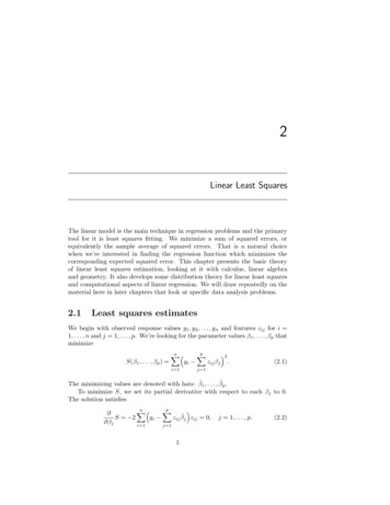
Transcription
2Linear Least SquaresThe linear model is the main technique in regression problems and the primarytool for it is least squares fitting. We minimize a sum of squared errors, orequivalently the sample average of squared errors. That is a natural choicewhen we’re interested in finding the regression function which minimizes thecorresponding expected squared error. This chapter presents the basic theoryof linear least squares estimation, looking at it with calculus, linear algebraand geometry. It also develops some distribution theory for linear least squaresand computational aspects of linear regression. We will draw repeatedly on thematerial here in later chapters that look at specific data analysis problems.2.1Least squares estimatesWe begin with observed response values y1 , y2 , . . . , yn and features zij for i 1, . . . , n and j 1, . . . , p. We’re looking for the parameter values β1 , . . . , βp thatminimizeS(β1 , . . . , βp ) n Xi 1yi pXzij βj 2.(2.1)j 1The minimizing values are denoted with hats: β̂1 , . . . , β̂p .To minimize S, we set its partial derivative with respect to each βj to 0.The solution satisfiespn XX S 2yi zij β̂j zij 0, βji 1j 11j 1, . . . , p.(2.2)
22. LINEAR LEAST SQUARESWe’ll show later that this indeed gives the minimum, not the maximum or asaddle point. The p equations in (2.2) are known as the normal equations.This is due to normal being a synonym for perpendicular or orthogonal, andnot due to any assumption about the normal distribution. Consider the vectorZ j (z1j , . . . , znj )0 Rn of values for the j’th feature. Equation (2.2) saysthat this feature vector Phas a dot product of zero with the residual vector havingpi’th element ε̂i yi j 1 zij β̂j . Each feature vector is orthogonal (normal)to the vector of residuals.It is worth while writing equations (2.1) and (2.2) in matrix notation. Thoughthe transition from (2.1) to (2.2) is simpler with coordinates, our later manipulations are easier in vector form. Let’s pack the responses and feature valuesinto the vector Y and matrix Z via y1z11 z12 . . . z1p y2 z21 z22 . . . z2p Y . , and, Z . . . . ynzn1 zn2 . . . znpWe also put β (β1 , . . . , βp )0 and let β̂ denote the minimizer of the sum ofsquares. Finally let ε̂ Y Z β̂, the n vector of residuals.Now equation (2.1) can be written S(β) (Y Zβ)0 (Y Zβ) and thenormal equations (2.2) becomeε̂0 Z 0(2.3)after dividing by 2. These normal equations can also be writtenZ 0 Z β̂ Z 0 Y.(2.4)When Z 0 Z is invertible then we find thatβ̂ (Z 0 Z) 1 Z 0 Y.(2.5)We’ll suppose at first that Z 0 Z is invertible and then consider the singular casein Chapter 2.7.Equation (2.5) underlies another meaning of the work ‘linear’ in linear regression. The estimated coefficient β̂ is a fixed linear combination of Y , meaningthat we get it by multiplying Y by the matrix (Z 0 Z) 1 Z 0 . The predicted valueof Y at any new point x0 with features z0 φ(x0 ) is also linear in Y ; it isz00 (Z 0 Z) 1 Z 0 Y .Now let’s prove that β̂ (Z 0 Z) 1 Z 0 Y is in fact the minimizer, not just apoint where the gradient of the sum of squares vanishes. It seems obvious thata sum of squares like (2.1) cannot have a maximizing β. But we need to ruleout saddle points too, and we’ll also find that β̂ is the unique least squaresestimator. Since we already found an expression for β̂ we prove it is right byexpressing a generic βe Rp as β̂ (βe β̂) and then expanding S(β̂ (βe β̂)).This adding and subtracting technique is often applicable in problems featuringsquared errors.
2.2. GEOMETRY OF LEAST SQUARES3Theorem 2.1. Let Z be an n p matrix with Z 0 Z invertible, and let Y be ann vector. Define S(β) (Y Zβ)0 (Y Zβ) and set β̂ (Z 0 Z) 1 Z 0 Y . ThenS(β) S(β̂) holds whenever β 6 β̂.Proof. We know that Z 0 (Y Z β̂) 0 and will use it below. Let βe be any pointin Rp and let γ βe β̂. Thene (Y Z β)e 0 (Y Z β)eS(β) (Y Z β̂ Zγ)0 (Y Z β̂ Zγ) (Y Z β̂)0 (Y Z β̂) γ 0 Z 0 (Y Z β̂) (Y Z β̂)Zγ γ 0 Z 0 Zγ S(β̂) γ 0 Z 0 Zγ.e S(β̂) kZγk2 S(β̂). It follows that β̂ is a minimizer of S.Thus S(β)For uniqueness we need to show that γ 6 0 implies Zγ 6 0. Suppose to thecontrary that Zγ 0 for γ 6 0. Then we would have Z 0 Zγ 0 for γ 6 0, butthis contradicts the assumption that Z 0 Z is invertible. Therefore if βe 6 β̂ thene S(β̂) kZ(βe β̂)k2 0S(β)2.2Geometry of least squaresFigure xxx shows a sketch to illustrate linear least squares. The vector y (y1 , . . . , yn )0 is represented as a point in Rn . The setM {Zβ β Rp }(2.6)is a p dimensional linear subset of Rn . It is fully p dimensional here becausewe have assumed that Z 0 Z is invertible and so Z has rank p. Under our model,E(Y ) Zβ M.The idea behind least squares is to find β̂ so that ŷ Z β̂ is the closest pointto y from within M. We expect to find this closest point to y by “dropping aperpendicular line” to M. That is, the error ε̂ y ŷ should be perpendicularto any line within M. From the normal equations (2.3), we have ε̂0 Z 0 so ε̂is actually perpendicular to every point Zβ M. Therefore ε̂ is perpendicularto every line in M.We can form a right angle triangle using the three points y, ŷ and Z βe forany βe Rp . Taking βe 0 and using Pythagoras’ theorem we getkyk2 kε̂k2 kz β̂k2 .When the first column of Z consists of 1s then (ȳ, . . . , ȳ)0 Z(ȳ, 0, . . . , 0) Mand Pythagoras’ theorem impliesnnnXXX(yi ȳ)2 (ŷi ȳ)2 (yi ŷ)2 .i 1i 1i 1(2.7)
42. LINEAR LEAST SQUARESThe left side of (2.7) is called the centered sum of squares of the yi . It isn 1 times the usual estimate of the common variance of the Yi . The equationdecomposes this sum of squares into two parts. The first is the centered sum ofsquared errors of the fitted values ŷi . The second is the sumPof squared modelnerrors. When the first column of Z consists of 1s then (1/n) i 1 ŷi ȳ. That is ŷ ȳ. Now the two terms in (2.7) correspond to the sum of squares of thefitted values ŷi about their mean and the sum of squared residuals. We writethis as SSTOT SSFIT SSRES . The total sum of squares is the sum of squaredfits plus the sum of squared residuals.Some of the variation in Y is ‘explained’ by the model and some of it leftunexplained. The fraction explained is denoted byR2 SSRESSSFIT 1 .SSTOTSSTOTThe quantity R2 is known as the coefficient of determination. It measures howwell Y is predicted or determined by Z β̂. Its nonnegative square root R is calledthe coefficient of multiple correlation. It is one measure of how well the responseY correlates with the p predictors in Z taken collectively. For the special caseof simple linear regression with zi (1, xi ) R2 then (Exercise xxx) R2 is thesquare of the usual Pearson correlation of x and y.Equation (2.7) is an example of an ANOVA (short for analysis of variance)decomposition. ANOVA decompositions split a variance (or a sum of squares)into two or more pieces. Not surprisingly there is typically some orthogonalityor the Pythagoras theorem behind them.2.3Algebra of least squaresThe predicted value for yi , using the least squares estimates, is ŷi Zi β̂. Wecan write the whole vector of fitted values as ŷ Z β̂ Z(Z 0 Z) 1 Z 0 Y . That isŷ Hy whereH Z(Z 0 Z) 1 Z 0 .Tukey coined the term “hat matrix” for H because it puts the hat on y. Somesimple properties of the hat matrix are important in interpreting least squares.By writing H 2 HH out fully and cancelling we find H 2 H. A matrixH with H 2 H is called idempotent. In hindsight, it is geometrically obviousthat we should have had H 2 H. For any y Rn the closest point to y insideof M is Hy. Since Hy is already in M, H(Hy) Hy. That is H 2 y Hy forany y and so H 2 H. Clearly H k H for any integer k 1.The matrix Z 0 Z is symmetric, and so therefore is (Z 0 Z) 1 . It follows thatthe hat matrix H is symmetric too. A symmetric idempotent matrix such as His called a perpendicular projection matrix.Theorem 2.2. Let H be a symmetric idempotent real valued matrix. Then theeigenvalues of H are all either 0 or 1.
2.4. DISTRIBUTIONAL RESULTS5Proof. Suppose that x is an eigenvector of H with eigenvalue λ, so Hx λx.Because H is idempotent H 2 x Hx λx. But we also have H 2 x H(Hx) H(λx) λ2 x. Therefore λx λ2 x. The definition of eigenvector does not allowx 0 and so we must have λ2 λ. Either λ 0 or λ 1.Let H P 0 ΛP Pwhere the columns of P are eigenvectors pi of H for i n1, . . . , n. Then H i 1 λi pi p0i , where by Theorem 2.2 each λi is 0 or 1. Withno loss of generality, we can arrangethe ones to precede the zeros. SupposePforrthat there are r ones. Then H i 1 pi p0i . We certainly expect r to equal phere. This indeed holds. The eigenvalues of H sum to r, so tr(H) r. Alsotr(H)P tr(Z(Z 0 Z) 1 Z 0 ) tr(Z 0 Z(Z 0 Z) 1 ) tr(Ip ) p. Therefore r p andpH i 1 pi p0i where pi are mutually orthogonal n vectors.The prediction for observation i can be written as ŷi Hi y where Hi isthe i’th row of the hat matrix. The i’th row of H is simply zi0 (Z 0 Z) 1 Z 0 andthe ij element of the hat matrix is Hij zi0 (Z 0 Z) 1 zj . Because Hij Hji thecontribution of yi to ŷj equals that of yj to ŷi . The diagonal elements of thehat matrix will prove to be very important. They areHii zi0 (Z 0 Z) 1 zi .(2.8)We are also interested in the residuals ε̂i yi ŷi . The entire vector ofresiduals may be written ε̂ y ŷ (I H)y. It is easy to see that ifH is a PPM, then so is I H. Symmetry is trivial, and (I H)(I H) I H H HH I H.pThe model space M {Zβ β RP} is the set of linear combinations ofpcolumns of Z. A typical entry of M is j 1 βj Z j . Thus M is what is knownas the column space of Z, denoted col(Z). The hat matrix H projects vectorsonto col(Z). The set of vectors orthogonal to Z, that is with Zv 0, is a linearsubspace of Rn , known as the null space of Z. We may write it as M or asnull(Z). The column space and null spaces are orthogonal complements. Anyv Rn can be uniquely written as v1 v2 where v1 M and v2 M . Interms of the hat matrix, v1 Hv and v2 (I H)v.2.4Distributional resultsWe continue to suppose that X and hence Z is a nonrandom matrix and thatZ has full rank. The least squares model has Y Zβ ε. Thenβ̂ (Z 0 Z) 1 Z 0 Y (Z 0 Z) 1 (Z 0 Zβ ε) β (Z 0 Z) 1 Z 0 ε.(2.9)The only randomness in the right side of (2.9) comes from ε. This makes it easyto work out the mean and variance of β̂ in the fixed x.Lemma 2.1. If Y Zβ ε where Z is nonrandom and Z 0 Z is invertible andE(ε) 0, thenE(β̂) β.(2.10)
62. LINEAR LEAST SQUARESProof. E(β̂) β (Z 0 Z) 1 Z 0 E(ε) β.The least squares estimates β̂ are unbiased for β as long as ε has meanzero. Lemma 2.1 does not require normally distributed errors. It does not evenmake any assumptions about var(ε). To study the variance of β̂ we will needassumptions on var(ε), but not on its mean.Lemma 2.2. If Y Zβ ε where Z is nonrandom and Z 0 Z is invertible andvar(ε) σ 2 I, for 0 σ 2 , thenvar(β̂) (Z 0 Z) 1 σ 2 .(2.11)Proof. Using equation (2.9),var(β̂) (Z 0 Z) 1 Z 0 var(ε)Z(Z 0 Z) 1 (Z 0 Z) 1 Z 0 σ 2 I Z(Z 0 Z) 1 (Z 0 Z) 1 σ 2 ,(2.12)after a particularly nice cancellation.We will look at and interpret equation (2.12) for many specific linear models. For now we notice that it holds without regard to whether ε is normallydistributed or even whether it has mean 0.Up to now we have studied the mean and variance of the estimate of β. Nextwe turn our attention to σ 2 . The key to estimating σ 2 is the residual vector ε̂.Lemma 2.3. Under the conditions of Lemma 2.2, E(ε̂0 ε̂) (n p)σ 2 . Forp n the estimatens2 1 X(Yi zi0 β̂)2n p i 1(2.13)satisfies E(s2 ) σ 2 .Proof. Recall that ε̂ (I H)ε. Therefore E(ε̂0 ε̂) E(ε0 (I H)ε) tr((I H)Iσ 2 ) (n p)σ 2 . Finally s2 ε̂0 ε̂/(n p).Now we add in the strong assumption that ε N (0, σ 2 I). Normally distributed errors make for normally distributed least squares estimates, fits andresiduals.Theorem 2.3. Suppose that Z is an n by p matrix of real values, Z 0 Z isinvertible, and Y Zβ ε where ε N (0, σ 2 I). Thenβ̂ N (β, (Z 0 Z) 1 σ 2 ),ŷ N (Zβ, Hσ 2 ),ε̂ N (0, (I H)σ 2 ),where H Z(Z 0 Z) 1 Z 0 . Furthermore, ε̂ is independent of β̂ and of ŷ.
2.4. DISTRIBUTIONAL RESULTS7Proof. Consider the vector 0 1 0 (Z Z) Zβ̂ Y Rp 2n .Hv ŷ I Hε̂The response Y has a multivariate normal distribution and so therefore does v.Hence each of β̂, ŷ, and ε̂ is multivariate normal.The expected value of v is 0 1 0 (Z Z) Zββ Zβ HZβ Zβ HE(v) I H(I H)Zβ0because HZ Z, establishing the means listed above for β̂, ŷ and ε̂.The variance of β̂ is (Z 0 Z) 1 σ 2 by Lemma 2.2. The variance of ŷ is var(ŷ) Hvar(Y )H 0 H(σ 2 I)H Hσ 2 because H is symmetric and idempotent. Similarly ε̂ (I H)(Zβ ε) (I H)ε and so var(ε̂) (I H)(σ 2 I)(I H)0 (I H)σ 2 because I H is symmetric and idempotent.We have established the three distributions displayed but have yet to provethe claimed independence. To this endcov(β̂, ε̂) (Z 0 Z) 1 Z 0 (σ 2 I)(I H) (Z 0 Z) 1 (Z HZ)0 σ 2 0because Z HZ. Therefore β̂ and ε̂ are uncorrelated and hence independentbecause v has a normal distribution. Similarly cov(ŷ, ε̂) H(I H)0 σ 2 (H HH 0 )σ 2 0 establishing the second and final independence claim.We can glean some insight about the hat matrix from Theorem 2.3. Firstbecause var(ŷi ) σ 2 Hii we have Hii 0. Next because var(ε̂) σ 2 (1 Hii )we have 1 Hii 0. Therefore 0 Hii 1 holds for i 1, . . . , n.Theorem 2.4.conditions of Theorem 2.3, and also that p n.PnAssume the102Let s2 n p(Y zβ̂). Theniii 1(n p)s2 σ 2 χ2(n p) .(2.14)Proof. First(n p)s2 (Y Z β̂)0 (Y Z β̂) Y 0 (I H)Y ε0 (I H)ε.The matrix I H can be written I H P ΛP
squared errors of the tted values y i. The second is the sum of squared model errors. When the rst column of Zconsists of 1s then (1 n) P n i 1 y i y. That is y y. Now the two terms in (2.7) correspond to the sum of squares of the tted values y i about their mean and the sum of squared

