Transcription
Efficient Similarity Estimation for SystemsExploiting Data RedundancyKanat Tangwongsan1 , Himabindu Pucha2 , David G. Andersen1 , Michael Kaminsky31Carnegie Mellon University, 2 IBM Research Almaden, 3 Intel Labs PittsburghAbstract—Many modern systems exploit data redundancy toimprove efficiency. These systems split data into chunks, generateidentifiers for each of them, and compare the identifiers amongother data items to identify duplicate chunks. As a result, chunksize becomes a critical parameter for the efficiency of these systems: it trades potentially improved similarity detection (smallerchunks) with increased overhead to represent more chunks.Unfortunately, the similarity between files increases unpredictably with smaller chunk sizes, even for data of the same type.Existing systems often pick one chunk size that is “good enough”for many cases because they lack efficient techniques to determinethe benefits at other chunk sizes. This paper addresses thisdeficiency via two contributions: (1) we present multi-resolution(MR) handprinting, an application-independent technique thatefficiently estimates similarity between data items at differentchunk sizes using a compact, multi-size representation of thedata; (2) we then evaluate the application of MR handprints toworkloads from peer-to-peer, file transfer, and storage systems,demonstrating that the chunk size selection enabled by MRhandprints can lead to real improvements over using a fixed chunksize in these systems.I. I NTRODUCTION“We were most concerned about the choice of [chunk size]”–Spring & Wetherall [22]Exploiting cross-file redundancy has become an importanttechnique to improve the efficiency of data transfer and storage—so much so that just recently, a filesystem “deduplication”company (Data Domain) was acquired for over two billiondollars. Redundancy elimination is widely used at the packetlevel (e.g., Spring and Wetherall [22], and WAN optimizersfrom companies such as Riverbed [21]); at the protocol level(e.g., Web page duplicate elimination [20]); for local [9] andremote filesystems (LBFS [13]); and for file transfers (rsyncand several peer-to-peer systems [1, 6, 16]). In general, thesesystems identify chunks of data shared across files, in order totransfer or store them more efficiently.For this reason, these systems all face the question of howto divide data into chunks. The goal of this chunking is tomaximize the probability of finding common chunks whileminimizing the overhead of transmitting and looking up chunkidentifiers. Choosing the correct chunk size is a fundamentaldecision in managing this tradeoff. Existing systems choose astatic value based upon one or a few intended data sets, andthe range of these values spans several orders of magnitude:SystemChunk SizeeMule (p2p)BitTorrent (p2p)SET (p2p)LBFS (dist. fs)Shark (dist. fs)REBL (filesystem)RsyncPacket-level9500 KB256 KB16 KB8 KB8 KB1 KB–8 KBVariable64 bytesIn this work, we study a seemingly simple question, andprovide a general-purpose technique and an empirical evaluationto help applications navigate this tradeoff: how can two or moreentities efficiently determine the best chunk size to use whentransferring/storing data?Answering this question is both challenging and important.It is challenging because doing so efficiently requires improvingupon previous work in similarity estimation. It is importantbecause a poor chunk size selection harms efficiency: too largea chunk size reduces the exploitable redundancy between files,but too small a chunk size can greatly increase the overhead ofrepresenting and transferring the file. Unfortunately, the rightchunk size can vary dramatically even within files of the sametype.To illustrate this point, consider an example from a realp2p file-sharing network: One popular English movie was 75%similar to the same movie in Italian using 1 KByte chunks,but only 3% similar using 128 KByte chunks. The movieshave identical video streams, but different audio streams. Thus,the chunk size needs to be smaller than a single video frameto decouple audio and video. The difference in overhead isalso large between small and large chunk sizes: A common800 MByte movie in 1 KByte chunks has 800,000 chunks,each of which must be requested and accounted for separately.Using BitTorrent’s 256 KByte chunk size, however, the samefile would be represented as only 3,125 chunks.Our solution involves an application-independent techniquethat efficiently estimates achievable benefit at different chunksizes, a building block for optimal chunk size selection. Thealgorithm builds upon prior work in similarity detection [12,2, 3]; its key contribution is providing bounds on the sizeof the handprints that must be compared in order to obtainaccurate estimates, and using these bounds to design estimationtechniques that have very low overhead. It operates using acompact, multi-size representation of the data’s content, calleda multi-resolution (MR) handprint. We show analytically theerror bounds on such an estimate and provide theoretical results
indicating how many chunks must be included in the MRhandprint, at different sizes, so that the similarity estimate fallswithin those bounds (Sections III, IV). Although the techniquespresented here are not tied to any particular chunking scheme,in this paper, we focus on Rabin-based chunking and in thisparticular case, a chunk size refers to the expected chunk size.We empirically evaluate our algorithm using workloads froma p2p file system and an RPM/ISO mirror site. Our resultssuggest that an MR-handprint consuming 0.15% of the size ofthe file can be used to estimate to within 5% (and often muchmore closely) the similarity between two files at chunk sizesof 1, 2, 4, ., 128 KBytes (plausible chunk sizes in a p2p filetransfer system).We then illustrate the utility of multi-resolution handprintingin both our workloads. As discussed in Section V, in the p2pscenario, MR-handprinting identifies that only a small fractionof files actually benefit the most at a static chunk size of16 KBytes (as used in [16]); 40% of the file transfers wouldhave higher performance with larger chunk sizes, and 60% ofthe transfers would have higher performance with chunk sizessmaller than 16 KBytes. Similarly, in the RPM/ISO scenario, 20% of files can be transferred faster with a larger chunksize, while 80% of files benefit from smaller chunk sizes.II. M OTIVATION AND BACKGROUNDA. Why different chunk sizes?We motivate this work by presenting the observation thatled to this research: the drastically different similarity observedat different chunk sizes for different types of objects, and fordifferent objects of the same type. We first examine a handfulof example files sampled from a p2p file sharing system and acollection of ISO/RPM files to understand similarity at differentchunk sizes; we examine a larger collection of files in Section V.We begin with two definitions:Splitting data into chunks: Rabin Fingerprinting. In thispaper, we adopt the now-common technique of dividing objectsinto chunks using content-determined boundaries, which renderthe chunk divisions insensitive to small insertions or deletions.This technique, termed Rabin fingerprinting and first used inLBFS [13], runs a sliding-window hash, covering about 40bytes, over the data, declaring a chunk boundary whenever thek-lowest-order bits of the hash (of those 40 bytes) are zero.For efficiency, it uses Rabin polynomial fingerprints as thehash [19]. The value of k determines the expected chunk size.1The effect of choosing boundaries based upon the content ofthe object is that an edit that adds or removes a small amountof data will only change the chunking in a local area of theobject, but the rest of the object will still have the same chunksas before.Similarity Metric. We define the similarity between two setsof chunks A and B as: A B s(A, B) A 1 We follow the LBFS example and also set a minimum and maximum chunksize as a function of the expected chunk size to bound the resulting chunksizes under pathological inputs.This definition matches the goals of a system exploitingredundancy—it is, in essence, a measure of how useful objectB is when trying to transfer/store object A. (This notion ofsimilarity, originally called containment, was proposed andstudied by Broder [2] and Broder et al. [3]).Similarity in Real-World Files: Figures 1(a), 1(b), and 1(c)show similarity vs. chunk size for a small set of audio, video,and software files, respectively. Each graph has four lines, witheach line showing how similar one pair of files was as thechunk size increases from 1 KByte to 128 KBytes.For instance, in the ISO/RPM files graph (Figure 1(c)), thetop line (Example 1) shows the similarity between two installdiscs for Yellowdog Linux, one from March 2003 and onefrom May 2003. In contrast, the line that drops drastically withchunk size (Example 2) is two source code RPMs of gcc, onegcc-2.96-128.7.2 and the other gcc-2.96-113.These graphs illustrate that among individual files, somehave roughly constant similarity across chunk sizes (and thus,could use a large chunk size to reduce overhead). Other files(e.g., Figure 1(a), example 3, and Figure 1(c), example 2) havesimilarity that “crashes” after a certain chunk size—but thatoptimal chunk size varies between different file types. Still,others have similarity that decreases more slowly, or linearly,with increasing chunk size.These were, of course, only sixteen example file pairs out ofthe entire universe of files that users may wish to transfer, butwe observe similar patterns in larger sets of files: In a largecollection of video files, a small number of files are nearly 200xmore similar at 1 KByte chunk size than they are at 128 KBytechunks. The decrease in video file similarity past 4–8 KBytes isstriking, because of the interleaving effect mentioned earlier. Incontrast, the similarity of audio files drops less sharply, becausemost similar audio files differ only in the first or last chunk.B. Example: P2P File TransfersTo provide context for the remainder of the paper, we brieflyoutline how we envision MR-handprints to be used in ourexample case study of p2p file transfer systems. This is neitherthe only use nor a complete design of a file-transfer systembased upon MR handprints. A file transfer system augmentedwith MR handprints will involve the following steps2 :(1) Identify candidate similar files (techniques proposed in [16]can be used);(2) Retrieve MR handprints for each candidate file;(3) Estimate similarity to desired file at different chunk sizes;(4) Determine the best chunk size to balance increased similarity with increased overhead;(5) Obtain the descriptor lists for the best chunk size; and(6) Transfer the file.In this context, our work focuses on providing tools for steps3 and 4 that keep the MR handprints small enough that step 2remains practical. The MR handprints can be compact becausethey are only used for similarity estimation. The descriptor listsused in the actual transfer still contain full hashes of the chunks(e.g., 160-bit SHA-1 hashes as used in [16]).2 Fordetails on a similarity based file transfer system, please refer to [16].
80806040200Example 1Example 2Example 3Example 410080Example 1Example 2Example 3Example 460Pair-wise similarity (%)100Pair-wise similarity (%)Pair-wise similarity (%)100402010100Example 1Example 2Example 3Example 44020016001Chunk size (KBytes)101001Chunk size (KBytes)(a) Audio files10100Chunk size (KBytes)(b) Video files(c) ISO and RPM filesFig. 1: Pair-wise similarity among files as chunk size is varied.III. E STIMATING S IMILARITYIn this section, we present a design for lightweight MRhandprints and show that they provide accurate estimates ofsimilarity. A MR-handprint is a compact representation of a dataitem (e.g., a file) with the property that given the MR-handprintsof any two data items, their similarity at all chunk sizes ofinterest can be estimated efficiently. Our method of generatinghandprints follows the work of Broder [2] for estimating bothour notion of similarity (which he calls containment) and theJaccard coefficient; however, Broder’s analysis did not providea comprehensive guideline for picking the parameters to controlthe accuracy and size of the resulting handprints. More recently,Pucha et al. [16] proposed a constant-size handprinting schemefor detecting whether two files share any chunk and give arecipe for controlling the size of the handprint while ensuringhigh accuracy. Their handprinting scheme, however, does notlead to accurate similarity estimates in our setting.Generating the multi-resolution handprint: The MR handprint contains, for each chunk size of interest, a subset of thehashes of the chunks in the data (e.g., a file). A chunk hashis included in the set if it is zero modulo some number k(e.g., if k 8, then, in expectation, 18 th of the chunk hasheswill be included in the handprint); i.e., for a set of hashes A,H(A) : {h A : h mod k 0}.Important to this definition is to note that inclusion in theset is a property of the chunk: if a chunk is in A’s handprint,that chunk will also be in the handprint of any file B that alsocontains the chunk. If the hash value of a chunk is effectivelyrandom (e.g., if the hash is secure), then any particular chunkessentially has a probability α 1/k of being included in thehandprint (independent of other chunks)3 .We vary α, which determines the handprint’s size, based uponthe chunk size for reasons we explain below. For implementationconvenience, we round up to the nearest power of two. Forexample, in a p2p file sharing system, α can be chosen asfollows:Chunk Size1KB2KB4KB8KB 16KBα1/161/81/41/213 Formally, each chunk e is associated with a Bernoulli random variablebe Be(α); we define H(A) {h A : bh 1}.These values are slightly more conservative than necessary(the fraction of chunks included could be somewhat smaller),but they produce highly accurate estimates while resulting inan MR-handprint that is only 0.15% the size of the file (using40-bit hashes as described in Section III-B).Estimating similarity using two handprints: The process issimple: Count the fraction of fingerprints in A’s handprint thatalso appear in B’s handprint. Use this fraction as an estimateof how similar A and B are. In other words,use A B H(A) H(B) as an estimate of H(A) A A. MR-Handprint AccuracyWe need to answer two key questions before using MRhandprinting in a system:(1) What fraction of chunk hashes should be included inthe handprint for a particular chunk size?(2) How accurate is the similarity estimate?More concretely, we wish to understand the probability thatthe estimated similarity differs from the true similarity by morethan a small amount δ. In particular, we study Pr [ bs s δ],where s is the true similarity, and sb the estimated similarity.The variable we control is α, the probability that a givenchunk is included in the handprint. By increasing this probability,we expect to decrease the error.We attack this problem in two ways. First, we numericallycompute the probability that an estimate is within δ for a fewvalues of δ, α, and A that we are particularly concernedwith. Because this numerical evaluation is computationallyintensive, we then derive a weaker, but tractable, lower boundon the confidence that can provide an understanding of howthe confidence scales with chunk size, the number of chunks,and α. (The theoretical bounds are also useful for estimatingconfidence for data whose size is too large to directly compute.)Confidence interval result summary: Table I shows theprobability that the similarity estimates are within 5% for alarge data item (32K chunks). Two things are clear: First, theconfidence values are high. Using a handprint that containsonly 1 chunk in 32 still results in an estimate that is within5% of the true value 98% of the time. Second, the theoretical
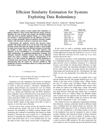
Inclusion Probability(α value)Confidence(bounds)Confidence(numerical) 1 0.9990.9820.7580.234 1 0.999 0.999 0.981 0.978α 1/2α 1/4α 1/8α 1/16α 1/32TABLE I: Confidence that similarity estimate is within 5% (δ 0.05)as the fraction of chunk hashes included in the MR-handprint varies(α). A 32, 768; files are 50% similar (s 0.5).Confidence Probability10.980.960.94within δ of the true similarity, as a function of the data size A , the true similarity s, and the fraction of chunk hashes inthe handprint α.Let us begin by stating a useful observation: the intersectionof the two handprints is the handprint of the intersection oftwo set of chunks (i.e., H(A) H(B) H(A B). This isbecause as noted earlier, inclusion in the handprint is a propertyof the chunk.Now we can lower-bound the confidence probability of theoverall estimate by bounding the error probability of two “badevents”—an excessive error in the denominator (the size of thehandprint of A) and in the numerator (the intersection of thetwo data items) of the similarity estimate—and then boundingthe probability that neither error occurs. Let λ be a parameterto be set later.(1) Bad event for denominator:E1 : { H(A) A α λ A α}0.920.900.20.40.60.81Similarity (s)Fig. 2: Numerically calculated confidence probability with 2048chunks, δ 0.05, and α 1/8.bound is not very tight for smaller values of α, but it providesa useful answer when the number of chunks is large: choosing118 or 16 th of the 1 KByte chunks provides very high confidencethat the estimate is within a few percent. As described later,using an MR-handprint with this fraction of chunks results inthe MR-handprint with 0.15% of the original content size,which seems a reasonable overhead.Directly calculating the confidence values: We derive anexpression for the probability that H(A) H(B) x and H(A) y. Let (1 s) A y A y s A f (x, y) α (1 α).xy xPThe confidence probability, then, is (x,y) Γ f (x, y), wherexΓ {(x, y) : s y δ, 0 y A , and y A\B x min(s A , y)}. To compute this exact confidence probability,we sum the probability of all possible outcomes in which theadditive error is at most δ. This calculation takes about 20minutes to perform for A 10, 000—fast enough for offlinecomputation, but too slow for on-line use. Since the computationtime grows rapidly with A , when the number of chunks islarge, we are limited to the theoretical bounds established inthe following section.To understand how the confidence probability varies withsimilarity level, Figure 2 shows the confidence probability atdifferent similarity level for A 2048 and α 1/8. Thelowest confidence is when s 0.5. We therefore use this valueof similarity in Table I.Confidence Bounds: We establish a theoretical bound forPr [ bs s δ], the probability that the similarity estimate is(2) Bad event for the numerator: Recall A B A s.E2 : { H(A B) A sα λ A sα}If neither bad event occurs, then the estimate error δ isδ/s2λless than 1 λs, so we set λ 2 δ/s. Note that the overallprobability of both conditions is at least the probability ofthem both occurring independently, and so we can calculatethe confidence probability as (1 Pr [E1 ])(1 Pr [E2 ]). This ispossible because the events E1 and E2 are negatively dependent—e.g., the size of A’s handprint must be larger than the size ofthe intersection of A and B’s handprint, so the probability ofE1 occurring, given that E2 occurred, is at least as high as theprobability of E1 occurring alone.Finally, we bound the above bad probabilities using theChernoff bounds, resulting in the following theorem:Theorem 1. Let λ is at least1 2e λ22δ/s22 δ/s2 .α A The probability Pr [ bs s δ]· (1 α) λ(1 2α)/3 1 2e λ22αs A · (1 α) λ(1 2α)/3 Proof Sketch. First, write the size of a handprint as a sum ofindicator random variables:XX H(A) 1{e H(A)} Xe ,e Ae Awhere Xe Be(α). Thus, E [ H(A) ] α A andE [ H(A) H(B) ] α A B . Then we lower bound
Efficient Similarity Estimation for Systems Exploiting Data Redundancy Kanat Tangwongsan 1, Himabindu Pucha2, David G. Andersen , Michael Kaminsky3 1Carnegie Mellon University, 2IBM Research Almaden, 3Intel Labs Pittsburg