Transcription
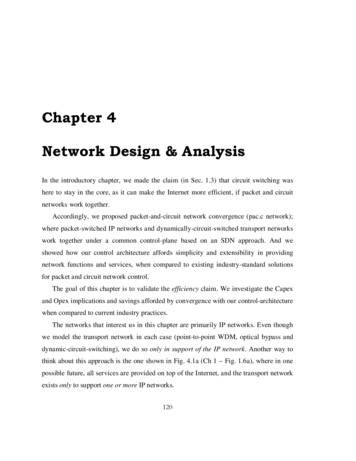
Chapter 4Network Design & AnalysisIn the introductory chapter, we made the claim (in Sec. 1.3) that circuit switching washere to stay in the core, as it can make the Internet more efficient, if packet and circuitnetworks work together.Accordingly, we proposed packet-and-circuit network convergence (pac.c network);where packet-switched IP networks and dynamically-circuit-switched transport networkswork together under a common control-plane based on an SDN approach. And weshowed how our control architecture affords simplicity and extensibility in providingnetwork functions and services, when compared to existing industry-standard solutionsfor packet and circuit network control.The goal of this chapter is to validate the efficiency claim. We investigate the Capexand Opex implications and savings afforded by convergence with our control-architecturewhen compared to current industry practices.The networks that interest us in this chapter are primarily IP networks. Even thoughwe model the transport network in each case (point-to-point WDM, optical bypass anddynamic-circuit-switching), we do so only in support of the IP network. Another way tothink about this approach is the one shown in Fig. 4.1a (Ch 1 – Fig. 1.6a), where in onepossible future, all services are provided on top of the Internet, and the transport networkexists only to support one or more IP networks.120
121Figure 4.1: (a) One possible future (b) Evaluation ProcedureOur approach to Capex and Opex analysis is as follows (Fig. 4.1b):1. We first outline a design methodology for a core IP network that is completelypacket-switched – i.e. all switching is performed by IP routers; and these routers areconnected over the wide-area by point-to-point WDM line systems. In other words,the transport network does not use any circuit switches to support the router-links andis completely static. This is in-fact the IP-over-WDM design scenario presented inSec. 1.3, and is a popular way for constructing core-IP networks today. We willconsider this as the reference design and model it in Sec 4.1.1.2. Next we consider a small variation of the reference design by adding optical-bypass.This is a technique by which the number of required core-router ports is reduced bykeeping transit-traffic in the optical domain (typically at a wavelength granularity).Optical bypass or express-links are used today in core-IP networks and also discussedin literature [79, 82, 83]. But it’s important to note that while optical-bypass can beachieved with optical switches, it is nevertheless a static approach – the opticalswitches do not switch wavelengths dynamically. IP over WDM with optical-bypassis modeled in Sec. 4.1.3.3. The first two steps cover industry-standard practices. In the final step we consider ourproposed network that uses both packet-switching and dynamic-circuit-switching(DCS) under a common control plane. While DCS can be used with IP in varying
122CHAPTER 4. NETWORK DESIGN & ANALYSISdegrees, we model an IP-and-DCS network with the following three characteristics:a) we replace Backbone Routers in PoPs with Backbone Packet-Optical Switches; b)we use a full-mesh of variable-bandwidth circuits between core-PoPs; and c) weadopt our unified control architecture for common control of packet and circuitswitching. In Sec. 4.2.2 we discuss these design choices and the motivation behindthem in terms of the benefits they afford when compared to the reference design; andwe outline the design methodology for such a converged network in Sec. 4.2.3.Analysis of our converged network (in Sec. 4.2.4) shows that we can achieve nearly60% lower Capex costs for switching hardware compared to the IP-over-WDM referencedesign; and 50% lower Capex compared to IP-over-WDM with static optical-bypass.Importantly, we show that while the savings achieved by optical-bypass (10-15%) can geteliminated if we vary the traffic-matrix, Capex savings in a pac.c network are insensitiveto varying traffic-matrices. Additionally, our design scales better (at a lower /Tbpsslope) when we scale the aggregate-traffic-demand from 1X to 5X. In Sec. 4.2.5, alimited Opex analysis that considers power-consumption, equipment-rack-rentals andnetwork-technician man-hours, shows nearly 40% in savings compared to the referencedesign.4.1Reference Design: IP over WDMThe core-IP network designed with an IP-over-WDM† approach can be modeled as acollection of routers in different city PoPs (Points-of-Presence). The backbone routers inthese PoPs are interconnected over the wide area by ‘waves’ (industry parlance) leasedfrom the transport network. Such waves are manifested by wavelengths stitched togetherin point-to-point WDM line-systems. There is no circuit-switching (static or dynamic) inthe transport network. In fact, in most cases, circuit-switches are not used at all toprovision these waves (which is what we model). As mentioned before, our focus is onArchitectural details were covered in Ch. 1- Sec. 1.4 and Ch 2 – Sec. 2.1 and 2.2.Unfortunately, such design is known by many names in the literature – IP over Optical [77], pure IP [79], IPover DWDM with TXP [83]. Others thankfully call it IP-over-WDM [84] †
123the IP network; we do not model the transport network individually; nor do we model theentire transport network ; and we do not consider other services or networks the transportnetwork might support today.It is worth noting that while our design methodology is detailed and comprehensive inits steps, it does not involve any optimization. No attempt has been made to optimize thedesign for any particular design criteria† , because optimization is not the goal here.Instead we wish to obtain ballpark-numbers for the relative comparison. As a result the IPnetwork is designed as a pure IP network sans any use of MPLS based traffic-engineeredtunnels.4.1.1Design MethodologyThe design methodology for IP-over-WDM design is briefly outlined below:1. Network Topologies: We choose representative topologies for both IP and WDMnetworks for a large US carrier like AT&T.2. Traffic-Matrix: We create a unidirectional (IP) traffic matrix from all cities in the IPtopology to all other cities in the topology. Each element in this matrix represents theaverage-traffic (in Gbps) sourced by one city and destined for the receiving-city.3. IP Edge-Dimensioning: In this step we account for all the traffic that could traversean edge in the IP topology. Such traffic includes a) the average traffic-demandbetween cities routed over the edge; b) traffic-rerouted over the edge in the event offailures; and c) head-room (over-provisioning) for variability in the traffic-volume inthe previous cases.4. IP PoP-Dimensioning: Once all the edges in the IP topology have been dimensioned,we calculate the number of parallel 10G links that make up the edge; and the numberof Backbone and Access Routers required in a PoP to switch between those links.5. WDM-Network Dimensioning: Finally each 10G link in the IP network is translatedto a wavelength path in the WDM network. The path is determined by routing theFor example, the transport network may be substantially bigger in terms of the number of switching nodes,compared to the IP network it supports (as highlighted in [77]).† Such design criteria could include the optimal routing of IP links to minimize concurrent failures, or the useof diverse-paths for routing, or the minimization of transponders in the transport network, etc.
124CHAPTER 4. NETWORK DESIGN & ANALYSIS(virtual) IP link over the WDM (fiber) topology. Once all IP links have been routed,we calculate the number of WDM line-systems, optical components and WDMtransponders required to satisfy the demand.Design Steps: We give more details and partial results for each step as follows:1. Network Topologies:a. We use AT&T’s IP network as reported by the Rocketfuel project (Fig. 4.2a)[78]†. The Rocketfuel topology gives us node-locations (cities) and edges (intercity connections). On this we layer typical PoP structure of access-routers (AR)dual-homed to two backbone routers (BR) (Fig. 4.2b). The ARs are either local(situated in same city PoP as the BRs) or housed in remote-cities [77]. The ARsaggregate traffic from the local and remote cities into the BRs, which areresponsible for switching traffic to other core-PoPs over the backbone edges. Thisstructure results in the hub-and-spoke look of Fig.4.2c; where the hubs are thecore city-PoPs (in 16 major cities); the spokes represent remote-sites (89 cities)that use remote-ARs to connect to the core-city PoP’s BRs; and 34 backboneedges that connect the BRs in the PoPs over the wide-area. Our use of the termedge to represent the wide-area inter-city connections will be resolved in thedimensioning process, into multiple parallel 10 Gbps IP links.b. For the WDM network, we use a topology from [79] shown in Fig.4.3a. Although[79] does not give details of the node-locations, we layer the topology on a map ofall North-American fiber routes [80] (Fig. 4.3b), to get the node locations andlink-distances. The fiber-topology includes 60 nodes and 77 edges, where thelongest edge-length is 1500 km and the average link length is 417km. Thephysical-edges of the WDM topology will be resolved in the dimensioningprocess into multiple parallel fibers and 40-wavelength C-band WDM linesystems.Note that network details (topology, number of switches, etc) are closely guarded secrets which carriers neverdivulge. The Rocketfuel project uses clever mechanisms to trace out network-topologies for several large ISPs.†
125(a)(b)(c)Figure 4.2: (a) AT&T’s IP network [78] (b) PoP structure (c) IP topology(a)(b)Figure 4.3: (a) Fiber (WDM) topology [79] (b) North-American Fiber Routes [80]
126CHAPTER 4. NETWORK DESIGN & ANALYSIS2. Unidirectional Traffic Matrix: We use a gravity-model as a starting point for a trafficmatrix [81]. For each of the 105 cities in the IP topology, we estimate the trafficsourced to the other 104 cities, by multiplying their populations and dividing by somepower of the physical-distance between them. Note that the power can be zero aswell, in which case distance is no longer a factor. We then scale the traffic-matrixentries to achieve a cumulative traffic-demand on the IP network of 2 Tbps†. Notethat this traffic matrix only considers the ISP’s internal traffic. It does not considerthe traffic to and from other-ISPs with which our ISP peers. Additionally, estimatingor predicting traffic matrices correctly is hard even for ISPs. Thus, later in theanalysis we vary the traffic matrix to study the effects on network Capex. We willalso scale the traffic matrix from 2X to 5X times the original aggregate demand, tostudy resultant effect on Capex and Opex.3. IP Edge-Dimensioning: This step is at the heart of the design process for the IPnetwork and is actually a combination of several steps:a. First the traffic-matrix is dimensioned on the core IP-network. Every demand inthe IP traffic-matrix is routed from source-AR to destination-AR over thebackbone IP topology (Fig. 4.2c). The route from source-AR to dest-AR is basedon Dijkstra’s shortest-path-first (SPF) algorithm, with the following assumptions:o Load-balancing (via ECMP) or traffic-engineering mechanisms (MPLS-TE)are not used.o The metric used in the SPF algorithm is hop-count*.The demand traffic is accounted for on each edge in the resultant shortest-pathroute. For example, in Fig. 4.4a, demand-traffic from AR1 to AR2, is routed viaBR1-BR3-BR2. Note that BR3 ‘sees’ this traffic as ‘transit’ traffic. The demandAR1 AR2 is tabulated on the core-edges between BR1 BR3 and BR3 BR2,and the access edges AR1 BR1 and AR2 BR2, accounting for direction oftraffic flow.From our discussion with ISPs, 2Tbps is a reasonable estimate of aggregate traffic demand on a UScontinental ISP’s core network, for fairly large carriers at the time of this writing (2011).* This is realistic – in the absence of any special metrics set by the network-operator for an edge in the IPtopology, routing protocols such as OSPF and IS-IS default to the same number for the routing metric for eachedge, effectively reducing the SPF calculation to a shortest-hop-count calculation. The metric for each edge isset by the network operator as an optimization, and as mentioned in the introduction we are not interested inoptimizing the design for any special purpose (which is also why we ignore ECMP and MPLS-TE)†
127(a)(b)Figure 4.4: Dimensioning the IP networkWe also keep track of the traffic ‘seen’ by the BRs in each PoP. From Fig. 4.4b,this includes the traffic switched locally between the ARs by the BRs; the trafficaggregated and ‘sourced-out’ by the BRs destined to other PoPs; the incomingtraffic from other PoPs destined to the ARs serviced by a PoP; and finally, thetraffic that transits through the BRs in a PoP, on their path to a destination PoP.b. Next, we account for failures by dimensioning for recovery. We break an edge inthe IP backbone-topology and re-route the entire traffic-matrix over the resultanttopology, which now has one less edge. Again this is precisely what wouldhappen as a result of individual Dijkstra calculations in every router in thenetwork. This time we get new values for the aggregate-traffic routed on eachedge of the failure-topology. By breaking each edge of the topology one-at-a-timeand tabulating the re-routed demands, we get different numbers for each edge forevery link-failure scenario. We then repeat this process by breaking each node inthe IP-core topology.oAssumption: We only consider single-failure scenarios – i.e if an edge in theIP topology breaks, no other IP edge or node breaks at the same time. If anode breaks, then transit through the node is not possible, but traffic can stillbe sourced in and out of the node due to dual-homing of ARs to BRs.
128CHAPTER 4. NETWORK DESIGN & ANALYSISoAssumption: We will see shortly that each edge in the IP topology is actuallyinstantiated by several parallel IP-links. We assume that the breakage of theedge corresponds to the breakage of all links that make up the edge.Neither assumption mentioned above is entirely true in practice, and depends onfactors such as the routing of the individual IP links over the underlying fibernetwork as well as the location and the cause of the failure. But to keep theanalysis simple and fair, we make the above assumptions and keep it consistentacross all design scenarios.c. At the end of the previous step, for each edge in the IP topology, we have thefollowing set of tabulated traffic in each direction– 1 for the original no-failuredemand-matrix, 34 link-failures and 16 node-failures (the max. of these is show inTable 4.1 for a few edges in the IP topology). For each edge we pick the highestaggregate out of all these cases for each direction. Then we pick the higher valuefrom the two directions, and set that as the bi-directional demand for each IP edge(last column in Table 4.1).BidirectionalDemand Demand Recovery max Recovery maxEdgeIP Edge-- --- -DimensionedChicago NewYork125.14130.36203.64220.89220.89LosAngeles Chicago97.3996.95118.28177.82177.82WashingtonDC NewYork97.1990.53133.31124.79133.31Orlando Atlanta91.7490.72177.40167.53177.40Atlanta WashingtonDC82.2571.16120.42108.07120.42Table 4.1: Routed traffic for a few IP edges (all values in Gbps)d. Finally we dimension for traffic variability by over-provisioning the edges. Suchover-provisioning can be performed by dividing the bi-directional traffic demandfrom the previous step, by an allowable-link-utilization factor [77]. We chose autilization factor of 25%, which translates into 4X over-provisioning.e. So far we have accounted for all backbone-edges (BR to BR). To account for theaccess-edges (AR to BR) we use the max. of the aggregate traffic sourced or sunk
129by the access-city. We account for failures by doubling this demand, as accesslinks are dual-homed to backbone routers. Finally we use the same overprovisioning factor we use in the backbone edges and set the resultant value as thebidirectional traffic-demand for the access edge.4. IP PoP-Dimensioning: Now that we have each edge of the IP network dimensionedfor demand, failures and traffic-variability, we can figure out the number of routers(ARs and BRs) in the PoPs and the number of links (or ports) that make up each edge(Fig. 4.5).Figure 4.5: Determining the Number of Routers and Linksa. The number of parallel access and backbone links (or interfaces) can bedetermined by simply dividing the edge demand by the linerate of a singleinterface (assumed 10Gbps for all interfaces).b. The number of access-routers in each access-city can be determined by summingup the number of access-to-BR interfaces, doubling it to account for aggregationinterfaces (assumed equal to the access-interfaces), multiplying by the line-rateand dividing by the AR switching-capacity (assumed 640 Gbps).c. The number of core-routers in each PoP is determined by summing up all theaccess and core interfaces, multiplying by the line-rate, and dividing by theswitching-capacity of a single BR (assumed 1.28 Tbps).
130CHAPTER 4. NETWORK DESIGN & ANALYSISCity PoPSeattleSanFranciscoLosAngelesNumber of Outgoing Parallel Links to BRs in other City PoPsChicago: 21, LosAngeles: 24, SanFrancisco: 3Chicago: 42, Dallas: 30, Denver: 2, LosAngeles: 34, StLouis: 9, Seattle:3Atlanta: 51, Chicago: 72, Dallas: 58, StLouis: 57, SanFrancisco: 34, Seattle: 24Table 4.2: Number of parallel IP Links making up an IP Edge for a few PoPs5. WDM Network-Dimensioning: In this step we route each IP-edge over the physicalfiber topology (Fig.4.6) to account for WDM network requirements.a. Again the IP edge is shortest-path routed over the fiber topology, but this time themetric used is the physical-distance of each edge in the fiber-topology (instead ofhop-count). Assumption: no optimization for routing IP edges on phy topology.IP link instantiatedby wavelength pathFigure 4.6: Routing an IP link on the Physical topologyb. The number of 10G interfaces calculated for the IP edge in the previous steptranslates into the number of 10G waves demanded from the WDM network. Thisdemand is then tabulated for each edge in the fiber topology over which the IPedge is routed. Assumption: all links that make up the IP edge are routed the sameway in the physical topology.c. Then on a per-physical-edge basis, we tabulate the aggregate ‘waves’ routed.From this we can figure out the number of parallel 40ch, C-band WDM linesystems required. For example, in Table 4.3, if the demand on a physical-edge is
131for 326 waves, 9 parallel line-systems would be required, with 8 of them fully-litand 1 partially lit (6 of the 40 waves will have transponders on either end).d. We also account for the number of line-systems required in series, by noting thelength of the physical-link and dividing it by the reach of the WDM line system.We assumed a line-system with 750km optical reach. Beyond 750km, the waveshave to be regenerated electronically using back-to-back transponders.Figure 4.7: WDM Line Systeme. Finally, we account for the optical components used in the fully and partially litsystems (Fig. 4.7). These include WDM transponders with client and line-sidetransceivers – the client-side connects to the router interfaces with short-reachoptics ( 2km) typically at the 1310nm wavelength; whereas the line-sidecontains long-reach optics at ITU grid wavelength (100s of km). The line-systemsalso contain wavelength multiplexers and de-multiplexers, pre/post and in-lineamplifiers (OLAs with a span of 80km), dispersion compensators (DCFs colocated with each amplifier) and dynamic gain-equalizers (DGEs co-located every4th amplifier). Table 4.3 shows results for a few edges in the fiber-topology.BidirectionalWaveLinkParallel lit-waves Full-reach Dist. ofPhysical EdgeDemand length(km) LineSysin lastSet of LS last (km)ElPaso Dallas32610278612
network is designed as a pure IP network sans any use of MPLS based traffic-engineered tunnels. 4.1.1 Design Methodology The design methodology for IP-over-WDM design is briefly outlined below: 1. Network Topolog ies: We choose representative topologies for both IP and WDM networks for a large US carrier like AT&T. 2.