Transcription
The 6% Ruleby Gerald C. Wagner, Ph.D.Gerald Wagner is President of Ibis Software, which specializes in reverse mortgages, and has beendescribed by Ken Scholen, of the AARP, as “the sharpest analytical mind we’ve seen in this market.” Hehas a Ph.D. in Economics from Harvard University. His thesis titled “Portfolio Construction andDiversification” was written under John Lintner, one of the founders of Modern Portfolio Theory.Executive SummaryThe 4% Rule appears to be alive and well. Advanced Monte Carlo simulations usingexpected asset class risks and returns that reflect the current economy show that the firstyear withdrawal can be increased by 2.5% each year and that portfolios with a 50% ormore equity exposure can give a 90% chance of “spending success” over 30 years.The cash proceeds from various reverse mortgage plans can be taken in various ways.Scheduled monthly tax-free advances reduce the need for portfolio withdrawals and cangive better “spending success” levels than line-of-credit draws.With a 30-year spending horizon and first-year withdrawal of 6.5%, reverse mortgagescheduled advances as a portfolio supplement give “spending success” levels of 91% –95%. Even with a first year withdrawal of 7.0%, success levels are still 85% – 89%.After 15 years, portfolio balances are materially higher, more than offsetting the homeequity being used by the reverse mortgage, i.e., overall net worth is higher.But is 30 years a long enough spending horizon? A couple in excellent health where thehusband is 65 years old and the wife is 63 years old, have a 42% chance that someonewill live past 30 years.Better planning would use a spending horizon where there is only a 10% chance thatsomeone is still alive. For this couple that would be 37 years from now.At 37 years, absent a reverse mortgage supplement, the 4% Rule becomes the 3.5% Rule.A 3.5% first-year draw can be increased by 2.5% each year and portfolios with a 50% ormore equity exposure can give a 86% – 92% chance of “spending success” over 37 yearsWith a 37-year spending horizon and first-year withdrawal of 6.0%, reverse mortgagescheduled advances as a portfolio supplement give “spending success” levels of 88% –92%. Even with a first year withdrawal of 6.5%, success levels are still 82% – 88%.The relative merits of using a reverse mortgage as a retirement spending supplementincrease as future portfolio expectations are lowered.Larry Bierwirth (1994) and William Bengen (1994) developed the 4% Rule which basically saysthat a person planning for a 30 year retirement, could withdraw 4% of their initial portfolio valuein the first year, increase those withdrawals each year for cost-of-living changes, and expect tohave a 90% chance of “spending success”. Spending success means that their portfolio would notbe depleted over the 30 year spending horizon. Bengen called this the “SAFEMAX” withdrawalrate.The order of portfolio returns is most important in spending success. If the portfolio experiencespoor performance in the early part of the spending horizon, it is difficult for it ever to recover.The retiree will likely run out of money. Conversely if the first years have good performance,
The 6% RulePage 2sticking with the 4% Rule will most often result in a large portfolio surplus at the end of 30years.Because the portfolio is stochastic, and the 4% Rule is static, it has been much maligned. Seeespecially Scott, Sharpe and Watson (2009). Several authors have suggested modifications suchas no inflation increases following bad portfolio years, etc. In reality, investment advisors,retirement planners, and the retirees themselves will assess the situation over time -- retirementitself is a stochastic process.A planner’s goal is to be able to sit down with a couple (or person), review their portfolio andother income sources, and create a plan that is both logical and explainable. That is why the 4%Rule has become so popular. This paper shows that it works well with portfolios that are at least50% invested in equities, and then shows how the use of a reverse mortgage can easily createnew rules like the 6.5% Rule for a 30 year horizon and the 6% Rule for a 37 year horizon.The primary reverse mortgage program available today is the FHA’s HECM (Home EquityConversion Mortgage). It comes in two versions: the Standard version includes a 2.0% FHAupfront mortgage insurance premium (MIP); the Saver version has only a de minimis upfrontMIP, but has benefits that are 15 to 20% lower. Salter, Pfeiffer, and Evensky (2012) discussedvarious ways to use the HECM Saver in retirement. Sacks (2012) discussed various ways to usethe HECM Standard line-of-credit as a supplement to portfolio withdrawals following a year ofin which the portfolio returns were less than the desired withdrawal.The HECM programs offer several ways of accessing the monies available. Upfront cash isneeded to pay off any liens against the home and can be drawn for any other purpose. Onecannot combine a reverse mortgage with a HELOC. A reverse mortgage must be in first position,and generally, does not allow any subordinate debt. With a reverse mortgage, a line-of-credit canbe accessed as desired. In a HECM, its capacity (limit) grows each year at the loan’s effectiveinterest rate. The growing line-of-credit capacity feature makes the HECM a very fair product.For example, with a note rate of 2.50% and ongoing MIP of 1.25% per annum, a loan’s effectiverate would be 3.75%. Imagine two borrower’s each with a 100,000 line-of-credit. One draws hisentire line-of-credit upfront; the other lets his line-of-credit capacity grow untouched for fiveyears. After five years the first borrower would owe 120,588 – that’s 100,000 in principal and 20,588 in accrued interest and MIP. The second borrower would owe nothing and have a lineof-credit capacity of 120,588. If he then withdrew his whole line-of-credit, both borrowerswould have the same outstanding loan balance.Reverse mortgages are due and payable when the home is no longer the principal residence ofthe borrower(s). By definition they are nonrecourse loans. With a HECM, if the accrued loanbalance exceeds the home value, the FHA insurance fund makes up the difference. Even if theloan is underwater, the heirs can buy the home for 95% of its then appraised value. It is acommon misconception that the bank owns the home. This is not true. The borrowers own thehome; they are responsible for maintaining the hazard insurance and paying the property taxes.Besides upfront cash and a line-of-credit, the HECM programs have two different payment planswith monthly advances to the borrower. One is called a Term plan wherein a certain amount isadvanced each month for a certain number of months. The advances then stop, but that does notmean the loan is due – it simply goes on accruing interest and MIP. The other payment plan is
The 6% RulePage 3called the Tenure plan (short for home tenure). This plan advances a certain amount each monthso long as the home is the principal residence of the borrower.For example, a 63-year old borrower with 250,000 available for a payment plan could receive 1,449 each month from a HECM tenure plan; that is 17,387 per year, and since these arenontaxable loan advances, their tax equivalent value is considerably higher. If the marginalfederal bracket was 28.0%, and they were in California (10.3%), the tax equivalent value of thesetenure advances would be 26,930. That works out to 10.8% per year on the 250,000 of theloan proceeds committed to this payment plan.If instead the same borrower wanted to use the 250,000 for a term plan over 15 years, themonthly loan advance would be 2,140 which is 25,686 per year in advances that have a taxequivalent value of 39,075. That works out to 15.9% per year on the 250,000 committed tothis term payment plan, but remember that advances will stop after 15 years. This paper showsthat reverse mortgage scheduled monthly payment plans can provide greater retirement spendingsuccess and higher expected future portfolio values than various methods that involve drawingon a line-of-credit. Payment plans should be much easier to explain to clients, and to manage,than calculating and varying the line-of-credit draws each year.The Model: All variables are stochastic and assumed to be log-normally distributed. Means andstandard deviations in the model can be set as you wish. In this paper it is estimated that futureannual home appreciation will be 3.0% with a 5.0% standard deviation; that the one-monthLIBOR will average an annual rate of 2.07% (currently it’s less than 0.25%) with a 0.53%standard deviation; and that annual future inflation (CPI–U) will average 2.50% with a 1.32%standard deviation.For future portfolio returns, Michaud (2012), a seasoned forecaster of future asset class risks andreturns, is used. In the model, the expected future return on an optimized portfolio with no equityexposure is 4.38% with a 9.90% standard deviation. The security market line ranges up to anexpected future return of 8.30% on a portfolio that is 100% in equities having a standarddeviation of 16.00%. These are nominal, not real returns. If future inflation averages 2.50% peryear, a nominal return of 8.30% indicates a real return on equities of 5.80%. This is not muchdifferent than the real return on equity used in Finke (2013), but Michaud’s 1.88% real return onfixed income is higher than that used in Finke. Pfau (2012) has an extensive literature review on safewithdrawal rates.Given one portfolio, one desired first-year draw rate, and one spending horizon, 2,000 MonteCarlo simulations were run across thirteen options. The first used the portfolio only with noreverse mortgage. Six were various plans using the HECM Standard, and six were various plansusing the HECM Saver. The various reverse mortgage plans are discussed below. For each runout of the 2,000 runs, four Monte Carlo arrays 50 years in length are created and used incalculating all 13 options. One array is the portfolio return, others are one-month LIBOR,inflation, and home appreciation. The 2,000 results are tabulated at the ‘spending horizon’. Theyare also tabulated at an intermediate year as few retired people remain in their home for 30 years.Across eight initial withdrawal rates ranging from 3.5% to 7.0%, across eight portfolios withequity exposure from 20% to 100%, and over two spending horizons (30 years and 37 years), thethirteen options required 1,664 Monte Carlo runs; each with 2,000 iterations -- and each iterationgoes though 20,000 formulas.
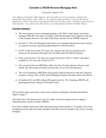
The 6% RulePage 4First the 4% Rule was tested to find how it and other withdrawal rates succeed across variousportfolio asset allocations. In Chart 1, the Red circle shows that portfolios that have equityexposure of 50% and higher reach close to or exceed the 90% success level predicted by the 4%Rule. Portfolios with less than 50% equity exposure have success levels commensurate with theirequity exposure. Note that the 4% withdrawal rate success of portfolios with equity exposure of50% and higher converge near the 90% success rate level. The extra volatility of the 100%equity portfolio makes its chances no better than the 80% equity portfolio.Chart 1Withdrawal Success - 30 Years - Portfolio Only100%90%Equities 0%3.50%4.00%4.50%5.00% 5.50% 6.00%Initial Withdrawal Rate6.50%7.00%Chart 1 shows that a portfolio that is 60% in equities has only a 30% chance of withdrawalsuccess if the initial withdrawal rate is 6.5% and grows, on average, by 2.5% each year. It willnow be shown that a 6.5% withdrawal rate can exceed 90% success with the use of a reversemortgage as a portfolio supplement.Supplement Portfolio Withdrawals with a Standard HECM Reverse MortgageSix ways of accessing funds from a reverse mortgage across a spending horizon of 30 years areexamined for a 63-year-old borrower living in a 450,000 home and having a 800,000retirement portfolio. The first year’s desired withdrawal is 6.5% which is 52,000. This is 4,333per month, and after paying federal and California taxes, leaves the homeowner with 2,798 tospend. The six HECM reverse mortgage possibilities are:Tenure Advances last as long as the home is the borrower’s primary residence. With the HECM,the monthly amount is calculated as a term loan to age 100. For the 63-year-old borrower that is444 months and produces 1,563 tax-free each month from the HECM. On a tax equivalent basisthat is 2,241, so to meet the desired withdrawal of 4,333, only 1,913 need be withdrawn fromthe portfolio each month during the first year. Since the HECM tenure advance is fixed, the
The 6% RulePage 5monthly portfolio withdrawal in the second year will be 2,021. The 108 increase over the firstyear accounts for the 2.5% expected annual inflation.Term Loan Advances Over the Spending Horizon changes the monthly advance calculations to360 months. The result is 1,662 which has a tax equivalent value of 2,574, so over the firstyear only 1,759 need be withdrawn for the portfolio each month. Since the HECM termadvance is fixed, the monthly portfolio withdrawal in the second year will be 1,867 to accountfor the 2.5% inflation.Term Loan First means setting up tax-free monthly HECM withdrawals of 2,798 so theportfolio need not be touched. It works out that a standard HECM can do this for 133 monthsbefore its capacity is exhausted. Since the HECM term advance is fixed, the monthly portfoliowithdrawal in the second year will be 108 to account for the 2.5% inflation. With the term loanfirst option, the portfolio can grow with only minimal withdrawals for 11.1 years. After that time100% of the spending money must come from the portfolio.Line-of-Credit Draws First is discussed by Sacks (2012). In the example, 2,798 is drawn fromthe HECM line-of-credit each month during the first year, and 2,868 is drawn from the line-ofcredit each month during the second year, etc. These withdrawals, growing each year withinflation, continue until the HECM is exhausted. The portfolio can remain untouched over thisperiod. However, as will shown, this ‘line-of-credit draws first’ option is dominated by the ‘termloan first’ option because of the method HECM calculates monthly loan advances.The note rate on a HECM varies each month based on the one-month LIBOR plus a set lender’smargin. The HECM pricing model uses the 10-year LIBOR swap rate as a proxy for the next 120months of the one-month LIBOR. Adding the lender’s margin, this 10-year rate is called theExpected Rate. Advances under Term and Tenure payment plans are calculated using thisExpected Rate plus the 1.25% MIP. But the line-of-credit grows only at the current 1-monthLIBOR plus margin plus the 1.25% MIP. Think of a car loan, higher rates mean higherpayments. That is why HECM scheduled payment plans dominate line-of-credit advances.For example, assume that 269,650 is available from a HECM reverse mortgage and that thespending horizon is 30 years. If the 10-year swap rate is 1.87% and margin is 2.50%, then theExpected Rate is 4.37%. A 30-year Term plan would give 1,544.17 each month. If the 1-monthLIBOR is 0.198% and margin is 2.50%, the Note Rate is 2.698%. So steady line-of-credit drawscould amount to only 1,275.08 each month. Thus, with today’s rates, a Term plan can pay out21% more than a line-of-credit plan. An inverted yield curve would reverse this effect.Since the current 1-month LIBOR is historically low, simulations in these notes use 2.07%, theaverage for the last ten years. We note that the monthly average for the 1-month LIBOR forSeptember, 2008, when Lehman Brothers fell, was 2.927%, and by January, 2009, the monthlyaverage had dropped to 0.383%. Interesting times.Line-of-Credit Draws with a Fixed Threshold such as -5% means that if the portfolio’s return lastyear was less than -5%, make the entire after-tax monthly withdrawal from the HECM line-ofcredit, for example the tax-free 2,798, and don’t touch the portfolio. However if the portfolioreturn was better than a loss of 5%, make the entire monthly withdrawal from the portfolio, forexample a taxable 4,333, and don’t touch the HECM. 20 thresholds of annual portfolio returnsranging from 90% to -90% were tested. In the Monte Carlo runs an annual portfolio return of 90% is never reached so the results are the same as HECM ‘line-of-credit draw first’. A -90%
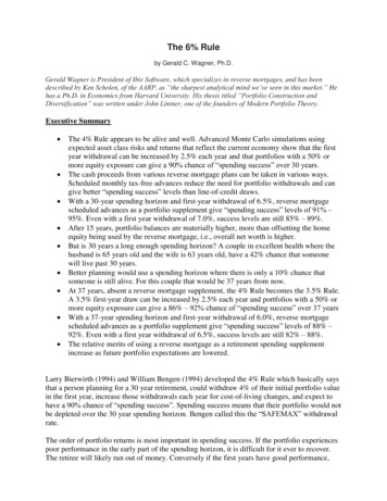
The 6% RulePage 6threshold, that’s minus 90% in one year, is always surpassed so the portfolio is always drawnfirst, and the HECM line-of-credit would be accessed only if and when the portfolio is depleted.As Sacks (2012) discusses, this ‘reverse mortgage last’ option has poor results. This is true.Sacks’ Coordinated Strategy consists of portfolio draws only from annual positive portfolioreturns. Any shortfall in the desired annual withdrawal is made up by drawing on the reversemortgage line-of-credit. When the reverse mortgage line-of-credit is exhausted, all withdrawalsare made from the portfolio regardless of its annual returns. See Sacks (2012) footnote 6.Chart 2 plots success rates for these six reverse mortgage options across various portfolios.Portfolios that are 60% or more invested in equities are very successful in meeting desiredwithdrawals. The sweet spot for spending success appears to be portfolios that are 70% investedin equities. Their chances of spending success range from 89.9% for the ‘line-of-credit drawfirst’ option up to 94.5% for the ‘term loan advances to spending horizon’ option. With thatoption, loan advances stop at the end of 30 years hence it bests the ‘tenure advances’ option.That’s because tenure advances are calculated to when the borrower will reach age 100. In thiscase that is 37 years. However tenure advances continue indefinitely, even if the homeownerlives to be 110. Using a 30-year spending horizon, no credit is given for those extra advances.If success over a spending horizon is all that matters, you can see that a portfolio need never beinvested in more than 70% equities. Bengen (1994) states that “Stock allocations below 50percent and above 75 percent are counterproductive.” It appears that he may be correct.100%Chart 230-Year Success Rates with 6.5% Initial WithdrawalTenureAdvances95%Term toHorizon90%Termadvance first85%LOC DrawFirst80%LOC -5.00%Trigger75%LOC SacksStrategy70%20%30%40%50%60%70%Percent in Equities80%90%100%30-year success rates are important to give your client a sense that their retirement planning issound. Average portfolio balances, home values, and loan balances have been calculated at thirtyyears; but thirty years is a long way off. As abundantly pointed out in the literature, if spending
The 6% RulePage 7withdrawals are successful over 30 years, there may be millions of dollars left on the table. Moremeaningful results would be those at some intermediate period, say fifteen years.Chart 3 shows the retirees expected net worth at the end of 15 years. This is the total of theirexpected portfolio balance and their remaining home equity. With the ‘Portfolio Only’ (noreverse mortgage) option, the home equity is the entire future home value. Obviously the highestportfolio balances result in the two options where the reverse mortgage is drawn first and theportfolio is allowed to grow with little or no withdrawals for much of the 15 years. The lowesttwo portfolio balances among the reverse mortgage options are those where the line of credit isused only intermittently. The less a reverse mortgage is utilized, the more is drawn for theportfolio, and hence, the lower the portfolio balance. Greater utilization of the reverse mortgagegives higher portfolio balances, but necessarily uses up home equity. You can see that the sixreverse mortgage options give higher overall results across all portfolio equity mixes than justrelying on the portfolio as the source of retirement spending.Chart 315-Year Portfolio Home Equity with 6.5% Initial
The primary reverse mortgage program available today is the FHA’s HECM (Home Equity Conversion Mortgage). It comes in two versions: the Standard version includes a 2.0% FHA upfront mortgage i