WIXLIB

INTRODUCTION TODIFFERENTIAL GEOMETRYJoel W. RobbinUW MadisonDietmar A. SalamonETH Zürich22 May 2021

ii

PrefaceThese are notes for the lecture course “Differential Geometry I” given by thesecond author at ETH Zürich in the fall semester 2017. They are based ona lecture course1 given by the first author at the University of Wisconsin–Madison in the fall semester 1983.One can distinguish extrinsic differential geometry and intrinsic differential geometry. The former restricts attention to submanifolds of Euclideanspace while the latter studies manifolds equipped with a Riemannian metric. The extrinsic theory is more accessible because we can visualize curvesand surfaces in R3 , but some topics can best be handled with the intrinsictheory. The definitions in Chapter 2 have been worded in such a way thatit is easy to read them either extrinsically or intrinsically and the subsequent chapters are mostly (but not entirely) extrinsic. One can teach a selfcontained one semester course in extrinsic differential geometry by startingwith Chapter 2, skipping the sections marked with an asterisk such as §2.8,and omitting the material in Chapter 7.This document is designed to be read either as a .pdf file or as a printedbook.We thank everyone who pointed out errors or typos in earlier versionsof this book. In particular, we thank Charel Antony and Samuel Trautweinfor many helpful comments.21 November 20191Joel W. Robbin and Dietmar A. SalamonExtrinsic Differential Geometryiii

iv

Contents1 What is Differential Geometry?1.1 Cartography and Differential Geometry1.2 Coordinates . . . . . . . . . . . . . . . .1.3 Topological Manifolds* . . . . . . . . . .1.4 Smooth Manifolds Defined* . . . . . . .1.5 The Master Plan . . . . . . . . . . . . .2 Foundations2.1 Submanifolds of Euclidean Space . . . . . . . . . . .2.2 Tangent Spaces and Derivatives . . . . . . . . . . . .2.2.1 Tangent Space . . . . . . . . . . . . . . . . .2.2.2 Derivative . . . . . . . . . . . . . . . . . . . .2.2.3 The Inverse Function Theorem . . . . . . . .2.3 Submanifolds and Embeddings . . . . . . . . . . . .2.4 Vector Fields and Flows . . . . . . . . . . . . . . . .2.4.1 Vector Fields . . . . . . . . . . . . . . . . . .2.4.2 The Flow of a Vector Field . . . . . . . . . .2.4.3 The Lie Bracket . . . . . . . . . . . . . . . .2.5 Lie Groups . . . . . . . . . . . . . . . . . . . . . . .2.5.1 Definition and Examples . . . . . . . . . . . .2.5.2 The Lie Algebra of a Lie Group . . . . . . . .2.5.3 Lie Group Homomorphisms . . . . . . . . . .2.5.4 Closed Subgroups . . . . . . . . . . . . . . .2.5.5 Lie Groups and Diffeomorphisms . . . . . . .2.5.6 Smooth Maps and Algebra Homomorphisms .2.5.7 Vector Fields and Derivations . . . . . . . . .2.6 Vector Bundles and Submersions . . . . . . . . . . .2.6.1 Submersions . . . . . . . . . . . . . . . . . .2.6.2 Vector Bundles . . . . . . . . . . . . . . . . 727274

viCONTENTS2.72.82.93 The3.13.23.33.43.53.63.7The Theorem of Frobenius . . . . . . . . . .The Intrinsic Definition of a Manifold* . . .2.8.1 Definition and Examples . . . . . . .2.8.2 Smooth Maps and Diffeomorphisms2.8.3 Tangent Spaces and Derivatives . . .2.8.4 Submanifolds and Embeddings . . .2.8.5 Tangent Bundle and Vector Fields .2.8.6 Coordinate Notation . . . . . . . . .Consequences of Paracompactness* . . . . .2.9.1 Paracompactness . . . . . . . . . . .2.9.2 Partitions of Unity . . . . . . . . . .2.9.3 Embedding in Euclidean Space . . .2.9.4 Leaves of a Foliation . . . . . . . . .2.9.5 Principal Bundles . . . . . . . . . .8087879293959799101101103107113114Levi-Civita ConnectionSecond Fundamental Form . . . . . . . . . . . . . .Covariant Derivative . . . . . . . . . . . . . . . . .Parallel Transport . . . . . . . . . . . . . . . . . .The Frame Bundle . . . . . . . . . . . . . . . . . .3.4.1 Frames of a Vector Space . . . . . . . . . .3.4.2 The Frame Bundle . . . . . . . . . . . . . .3.4.3 Horizontal Lifts . . . . . . . . . . . . . . . .Motions and Developments . . . . . . . . . . . . .3.5.1 Motion . . . . . . . . . . . . . . . . . . . .3.5.2 Sliding . . . . . . . . . . . . . . . . . . . . .3.5.3 Twisting and Wobbling . . . . . . . . . . .3.5.4 Development . . . . . . . . . . . . . . . . .Christoffel Symbols . . . . . . . . . . . . . . . . . .Riemannian Metrics* . . . . . . . . . . . . . . . . .3.7.1 Existence of Riemannian Metrics . . . . . .3.7.2 Two Examples . . . . . . . . . . . . . . . .3.7.3 The Levi-Civita Connection . . . . . . . . .3.7.4 Basic Vector Fields in the Intrinsic 166166169170173.1751751751781804 Geodesics4.1 Length and Energy . . . . . . . . . . . . . .4.1.1 The Length and Energy Functionals4.1.2 The Space of Paths . . . . . . . . . .4.1.3 Characterization of Geodesics . . . .

CONTENTS4.24.34.44.54.64.7viiDistance . . . . . . . . . . . . . . . . . . . . . . .The Exponential Map . . . . . . . . . . . . . . .4.3.1 Geodesic Spray . . . . . . . . . . . . . . .4.3.2 The Exponential Map . . . . . . . . . . .4.3.3 Examples and Exercises . . . . . . . . . .Minimal Geodesics . . . . . . . . . . . . . . . . .4.4.1 Characterization of Minimal Geodesics . .4.4.2 Local Existence of Minimal Geodesics . .4.4.3 Examples and Exercises . . . . . . . . . .Convex Neighborhoods . . . . . . . . . . . . . . .Completeness and Hopf–Rinow . . . . . . . . . .Geodesics in the Intrinsic Setting* . . . . . . . .4.7.1 Intrinsic Distance . . . . . . . . . . . . . .4.7.2 Geodesics and the Levi-Civita Connection4.7.3 Examples and Exercises . . . . . . . . . .1831911911921951971971992032052092172172192205 Curvature5.1 Isometries . . . . . . . . . . . . . . . . . . . . . . . .5.2 The Riemann Curvature Tensor . . . . . . . . . . . .5.2.1 Definition and Gauß–Codazzi . . . . . . . . .5.2.2 Covariant Derivative of a Global Vector Field5.2.3 A Global Formula . . . . . . . . . . . . . . .5.2.4 Symmetries . . . . . . . . . . . . . . . . . . .5.2.5 Riemannian Metrics on Lie Groups . . . . . .5.3 Generalized Theorema Egregium . . . . . . . . . . .5.3.1 Pushforward . . . . . . . . . . . . . . . . . .5.3.2 Theorema Egregium . . . . . . . . . . . . . .5.3.3 Gaußian Curvature . . . . . . . . . . . . . . .5.4 Curvature in Local Coordinates* . . . . . . . . . . .223. 223. 232. 232. 234. 237. 239. 241. 244. 244. 245. 249. 2546 Geometry and Topology6.1 The Cartan–Ambrose–Hicks Theorem . . . .6.1.1 Homotopy . . . . . . . . . . . . . . . .6.1.2 The Global C-A-H Theorem . . . . . .6.1.3 The Local C-A-H Theorem . . . . . .6.2 Flat Spaces . . . . . . . . . . . . . . . . . . .6.3 Symmetric Spaces . . . . . . . . . . . . . . .6.3.1 Symmetric Spaces . . . . . . . . . . .6.3.2 Covariant Derivative of the Curvature6.3.3 Examples and Exercises . . . . . . . .257257257259265268272273275278

viiiCONTENTS6.46.56.66.76.8Constant Curvature . . . . . . . . . . . . . .6.4.1 Sectional Curvature . . . . . . . . . .6.4.2 Constant Sectional Curvature . . . . .6.4.3 Hyperbolic Space . . . . . . . . . . . .Nonpositive Sectional Curvature . . . . . . .6.5.1 The Cartan–Hadamard Theorem . . .6.5.2 Cartan’s Fixed Point Theorem . . . .6.5.3 Positive Definite Symmetric Matrices .Positive Ricci Curvature* . . . . . . . . . . .Scalar Curvature* . . . . . . . . . . . . . . .The Weyl Tensor* . . . . . . . . . . . . . . .7 Topics in Geometry7.1 Conjugate Points and the Morse Index* . . . . . . .7.2 The Injectivity Radius* . . . . . . . . . . . . . . . .7.3 The Group of Isometries* . . . . . . . . . . . . . . .7.3.1 The Myers–Steenrod Theorem . . . . . . . .7.3.2 The Topology on the Space of Isometries . .7.3.3 Killing Vector Fields . . . . . . . . . . . . . .7.3.4 Proof of the Myers–Steenrod Theorem . . . .7.3.5 Examples and Exercises . . . . . . . . . . . .7.4 Isometries of Compact Lie Groups* . . . . . . . . . .7.5 Convex Functions on Hadamard Manifolds* . . . . .7.5.1 Convex Functions and The Sphere at Infinity7.5.2 Inner Products and Weighted Flags . . . . .7.5.3 Lengths of Vectors . . . . . . . . . . . . . . .7.6 Semisimple Lie Algebras* . . . . . . . . . . . . . . .7.6.1 Symmetric Inner Products . . . . . . . . . . .7.6.2 Simple Lie Algebras . . . . . . . . . . . . . .7.6.3 Semisimple Lie Algebras . . . . . . . . . . . .7.6.4 Complex Lie Algebras . . . . . . . . . . . . .280280281286293293299301308312318.325. 326. 336. 340. 340. 342. 345. 349. 358. 360. 365. 366. 374. 378. 388. 388. 391. 396. 401A Notes407A.1 Maps and Functions . . . . . . . . . . . . . . . . . . . . . . . 407A.2 Normal Forms . . . . . . . . . . . . . . . . . . . . . . . . . . . 408A.3 Euclidean Spaces . . . . . . . . . . . . . . . . . . . . . . . . . 410References413Index419

Chapter 1What is DifferentialGeometry?1.1Cartography and Differential GeometryCarl Friedrich Gauß (1777-1855) is the father of differential geometry. Hewas (among many other things) a cartographer and many terms in moderndifferential geometry (chart, atlas, map, coordinate system, geodesic, etc.)reflect these origins. He was led to his Theorema Egregium (see 5.3.1) bythe question of whether it is possible to draw an accurate map of a portionof our planet. Let us begin by discussing a mathematical formulation of thisproblem.Consider the two-dimensional sphere S 2 sitting in the three-dimensionalEuclidean space R3 . It is cut out by the equationx2 y 2 z 2 1.A map of a small region U S 2 is represented mathematically by a one-toone correspondence with a small region in the plane z 0. In this book wewill represent this with the notation φ : U φ(U ) R2 and call such anobject a chart or a system of local coordinates (see Fugure 1.1).What does it mean that φ is an “accurate” map? Ideally the user wouldwant to use the map to compute the length of a curve in S 2 . The length ofa curve γ connecting two points p, q S 2 is given by the formulaZ 1L(γ) γ̇(t) dt,γ(0) p, γ(1) q,0so the user will want the chart φ to satisfy L(γ) L(φ γ) for all curves γ.It is a consequence of the Theorema Egregium that there is no such chart.1

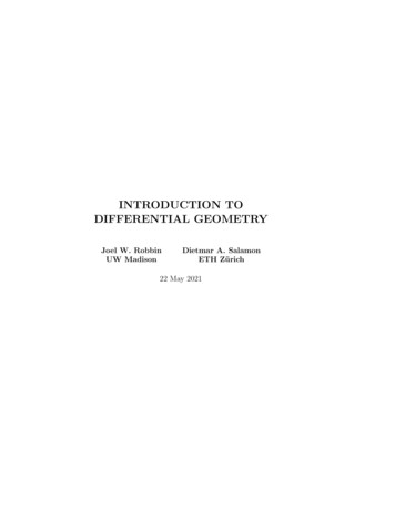
2CHAPTER 1. WHAT IS DIFFERENTIAL GEOMETRY?UφFigure 1.1: A chartPerhaps the user of such a map will be content to use the map to plotthe shortest path between two points p and q in U . This path is called ageodesic and is denoted by γpq . It satisfies L(γpq ) dU (p, q), wheredU (p, q) inf{L(γ) γ(t) U, γ(0) p, γ(1) q}so our less demanding user will be content if the chart φ satisfiesdU (p, q) dE (φ(p), φ(q))where dE (φ(p), φ(q)) is the length of the shortest path in the plane. It isalso a consequence of the Theorema Egregium that there is no such chart.Now suppose our user is content to have a map which makes it easy tonavigate close to the shortest path connecting two points. Ideally the userwould use a straight edge, magnetic compass, and protractor to do this.S/he would draw a straight line on the map connecting p and q and steer acourse which maintains a constant angle (on the map) between the courseand meridians. This can be done by the method of stereographic projection.This chart is conformal (which means that it preserves angles). Accordingto Wikipedia stereographic projection was known to the ancient Greeksand a map using stereographic projection was constructed in the early 16thcentury. Exercises 3.7.5, 3.7.12, and 6.4.22 use stereographic projection; thelatter exercise deals with the Poincaré model of the hyperbolic plane. Thehyperbolic plane provides a counterexample to Euclid’s Parallel Postulate.Exercise 1.1.1. It is more or less obvious that for any surface M R3there is a unique shortest path in M connecting two points if they aresufficiently close. (This will be proved in Theorem 4.5.3.) This shortestpath is called the minimal geodesic connecting p and q. Use this fact toprove that the minimal geodesic joining two points p and q in S 2 is an arcof the great circle through p and q. (This is the intersection of the spherewith the plane through p, q, and the center of the sphere.) Also prove thatthe minimal geodesic connecting two points in a plane is the straight line