WIXLIB

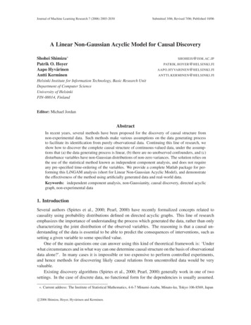
S HIMIZU , H OYER , H YV ÄRINEN AND K ERMINEN3. Model Identification Using Independent Component AnalysisThe key to the solution to the linear discovery problem is to realize that the observed variables arelinear functions of the disturbance variables, and the disturbance variables are mutually independentand non-Gaussian. If we as preprocessing subtract out the mean of each variable xi , we are left withthe following system of equations:x Bx e,(1)where B is a matrix that could be permuted (by simultaneous equal row and column permutations)to strict lower triangularity if one knew a causal ordering k(i) of the variables (Bollen, 1989). (Strictlower triangularity is here defined as lower triangular with all zeros on the diagonal.) Solving for xone obtainsx Ae,(2)where A (I B) 1 . Again, A could be permuted to lower triangularity (although not strict lowertriangularity, actually in this case all diagonal elements will be non-zero) with an appropriate permutation k(i). Taken together, Equation (2) and the independence and non-Gaussianity of the components of e define the standard linear independent component analysis model.Independent component analysis (ICA) (Comon, 1994; Hyvärinen et al., 2001) is a fairly recent statistical technique for identifying a linear model such as that given in Equation (2). If theobserved data is a linear, invertible mixture of non-Gaussian independent components, it can beshown (Comon, 1994) that the mixing matrix A is identifiable (up to scaling and permutation ofthe columns, as discussed below) given enough observed data vectors x. Furthermore, efficientalgorithms for estimating the mixing matrix are available (Hyvärinen, 1999).We again want to emphasize that ICA uses non-Gaussianity (that is, more than covariance information) to estimate the mixing matrix A (or equivalently its inverse W A 1 ). For Gaussiandisturbance variables ei , ICA cannot in general find the correct mixing matrix because many different mixing matrices yield the same covariance matrix, which in turn implies the exact same Gaussianjoint density (Hyvärinen et al., 2001). Our requirement for non-Gaussianity of disturbance variablesstems from the same requirement in ICA.While ICA is essentially able to estimate A (and W), there are two important indeterminacies that ICA cannot solve: First and foremost, the order of the independent components is in noway defined or fixed (Comon, 1994). Thus, we could reorder the independent components and,correspondingly, the columns of A (and rows of W) and get an equivalent ICA model (the sameprobability density for the data). In most applications of ICA, this indeterminacy is of no significance and can be ignored, but in LiNGAM, we can and we have to find the correct permutation asdescribed in Section 4 below.The second indeterminacy of ICA concerns the scaling of the independent components. In ICA,this is usually handled by assuming all independent components to have unit variance, and scalingW and A appropriately. On the other hand, in LiNGAM (as in SEM) we allow the disturbancevariables to have arbitrary (non-zero) variances, but fix their weight (connection strength) to theircorresponding observed variable to unity. This requires us to re-normalize the rows of W so thatall the diagonal elements equal unity, before computing B, as described in the LiNGAM algorithmbelow.Our discovery algorithm, detailed in the next section, can be briefly summarized as follows:First, use a standard ICA algorithm to obtain an estimate of the mixing matrix A (or equivalently2006

A L INEAR N ON -G AUSSIAN ACYCLIC M ODEL FOR C AUSAL D ISCOVERYof W), and subsequently permute it and normalize it appropriately before using it to compute Bcontaining the sought connection strengths bi j .34. LiNGAM Discovery AlgorithmBased on the observations given in Sections 2 and 3, we propose the following causal discoveryalgorithm:Algorithm A: LiNGAM discovery algorithm1. Given an m n data matrix X (m n), where each column contains one sample vector x, firstsubtract the mean from each row of X, then apply an ICA algorithm to obtain a decompositionX AS where S has the same size as X and contains in its rows the independent components.From here on, we will exclusively work with W A 1 .2. Find the one and only permutation of rows of W which yields a matrix W without any zeroson the main diagonal. In practice, small estimation errors will cause all elements of W to benon-zero, and hence the permutation is sought which minimizes i 1/ Wii .W by its corresponding diagonal element, to yield a new matrix W with all3. Divide each row of ones on the diagonal. of B using B I W .4. Compute an estimate B5. Finally, to find a causal order, find the permutation matrix P (applied equally to both rows and which yields a matrix B PBP T which is as close as possible to strictly lowercolumns) of B 2 .triangular. This can be measured for instance using i j BijA complete Matlab code package implementing this algorithm is available online at our LiNGAMhomepage: http://www.cs.helsinki.fi/group/neuroinf/lingam/We now describe each of these steps in more detail.In the first step of the algorithm, the ICA decomposition of the data is computed. Here, anystandard ICA algorithm can be used. Although our implementation uses the FastICA algorithm(Hyvärinen, 1999), one could equally well use one of the many other algorithms available (see e.g.,Hyvärinen et al., 2001). However, it is important to select an algorithm which can estimate independent components of many different distributions, as in general the distributions of the disturbancevariables will not be known in advance. For example, FastICA can estimate both super-Gaussianand sub-Gaussian independent components, and we don’t need to know the actual functional formof the non-Gaussian distributions (Hyvärinen, 1999).Because of the permutation indeterminacy of ICA, the rows of W will be in random order. Thismeans that we do not yet have the correct correspondence between the disturbance variables ei andthe observed variables xi . The former correspond to the rows of W while the latter correspond tothe columns of W. Thus, our first task is to permute the rows to obtain a correspondence betweenthe rows and columns. If W were estimated exactly, there would be only a single row permutation3. It would be extremely difficult to estimate B directly using a variant of ICA algorithms, because we don’t know thecorrect order of the variables, that is, the matrix B should be restricted to ‘permutable to lower triangularity’ not‘lower triangular’ directly. This is due to the permutation problem illustrated in Appendix B.2007

S HIMIZU , H OYER , H YV ÄRINEN AND K ERMINENthat would give a matrix with no zeros on the diagonal, and this permutation would give the correctcorrespondence. This is because of the assumption of DAG structure, which is the key to solvingthe permutation indeterminacy of ICA. (A proof of this is given in Appendix A, and an example ofthe permutation problem is provided in Appendix B.)In practice, however, ICA algorithms applied on finite data sets will yield estimates which areonly approximately zero for those elements which should be exactly zero, and the model is onlyapproximately correct for real data. Thus, our algorithm searches for the permutation using acost function which heavily penalizes small absolute values in the diagonal, as specified in step2. In addition to being intuitively sensible, this cost function can also be derived from a maximumlikelihood framework; for details, see Appendix C.When the number of observed variables xi is relatively small (less than eight or so) then findingthe best permutation is easy, since a simple exhaustive search can be performed. However, for higherdimensionalities a more sophisticated method is required. We also provide such a permutationmethod for large dimensions; for details, see Section 5.Once we have obtained the correct correspondence between rows and columns of the ICA decomposition, calculating our estimates of the bi j is straightforward. First, we normalize the rowsof the permuted matrix to yield a diagonal with all ones, and then remove this diagonal and flip thesign of the remaining coefficients, as specified in steps 3 and 4.Although we now have estimates of all coefficients bi j we do not yet have available a causalordering k(i) of the variables. Such an ordering (in general there may exist many if the generatingnetwork is not fully connected) is important for visualizing the resulting graph. A causal ordering can be found by permuting both rows and columns (using the same permutation) of the matrix B(containing the estimated connection strengths) to yield a strictly lower triangular matrix. If theestimates were exact, this would be a trivial task. However, since our estimates will not containexact zeros, we will have to settle for approximate strict lower triangularity, measured for instanceas described in step 5.4It has to be noted that the computational stability of our method cannot be guaranteed. This isbecause ICA estimation is typically based on optimization of non-quadratic, possibly non-convexfunctions, and the algorithm might get stuck in local minima. Thus, for different random initialpoints used in the optimization algorithm, we might get different estimates of W. An empiricalobservation is that typically ICA algorithms are relatively stable when the model holds, and unstable when the model does not hold. For a computational method addressing this issue, based onrerunning the ICA estimation part with different initial points, see Himberg et al. (2004).5. Permutation Algorithms for Large DimensionsIn this section, we describe efficient algorithms for finding the permutations in steps 2 and 5 of theLiNGAM algorithm. that would be zero in the4. A reviewer pointed out that from a Bayesian viewpoint, the non-zero entries of the matrix Binfinite data case manifest a more general concept: the data cannot identify ‘the’ DAG structure, they can only helpassign posterior probabilities to different structures.2008

A L INEAR N ON -G AUSSIAN ACYCLIC M ODEL FOR C AUSAL D ISCOVERY5.1 Permuting the Rows of WAn exhaustive search over all possible row-permutations is feasible only in relatively small dimensions. For larger problems other optimization methods are needed. Fortunately, it turns out that theoptimization problem can be written in the form of the classical linear assignment problem. To seethis set Ci j 1/ Wi j , in which case the problem can be written as the minimization ofm Cφ(i),i ,i 1where φ denotes the permutation to be optimized over. A great number of algorithms exist forthis problem, with the best achieving worst-case complexity of O(m3 ) where m is the number ofvariables (see e.g., Burkard and Cela, 1999).5.2 Permuting B to Get a Causal Order to yieldIt would be trivial to permute both rows and columns (using the same permutation) of Ba strictly lower triangular matrix if the estimates were exact, because one could use the followingalgorithm:Algorithm B: Testing for DAGness, and returning a causal order if true1. Initialize the permutation p to be an empty list contains no more elements:2. Repeat until B containing all zeros, if not possible return false(a) Find a row i of B(b) Append i to the end of the list p (c) Remove the i-th row and the i-th column from B3. Return true and the found permutation pHowever, since our estimates will not contain exact zeros, we will have to find a permutationsuch that setting the upper triangular elements to zero changes the matrix as little as possible. Forinstance, we could define our objective to be to minimize the sum of squares of elements on and 2 where B PBP T denotes the permuted B, and P denotes theabove the diagonal, that is i j Bijpermutation matrix representing the sought permutation. In low dimensions, the optimal permutation can be found by exhaustive search. However, for larger problems this is obviously infeasible.Since we are not aware of any efficient method for exactly solving this combinatorial problem, wehave taken another approach to handling the high-dimensional case.Our approach is based on setting small (absolute) valued elements to zero, and testing whetherthe resulting matrix can be permuted to strict lower triangularity. Thus, the algorithm is: by iterative pruning and testingAlgorithm C: Finding a permutation of B to zero1. Set the m(m 1)/2 smallest (in absolute value) elements of B2009

S HIMIZU , H OYER , H YV ÄRINEN AND K ERMINEN2. Repeat can be permuted to strict lower triangularity (using Algorithm B above). If the(a) Test if B , that is, B .answer is yes, stop and return the permuted B to zero(b) Additionally set the next smallest (in absolute value) element of B all the true zeros resulted in estimates smaller than all of the true nonIf in the estimated B,zeros, this algorithm finds the optimal permutation. In general, however, the result is not optimalin terms of the above proposed objective. However, simulations below show that the approximationworks quite well.6. Statistical Tests for Pruning EdgesThe LiNGAM algorithm consistently estimates the connection strengths (and a causal order) if themodel assumptions hold and the amount of data is sufficient. But what if our assumptions do not infact hold? In such a case there is of course no guarantee that the proposed discovery algorithm willfind true causal relationships between the variables.The good news is that, in some cases, it is possible to detect violations of the model assumptions. In the following sections, we provide three statistical tests: i) testing significance of bi j forpruning edges; ii) examining an overall fit of the model assumptions including estimated structureand connection strengths to data; iii) comparing two nested models. Then we propose a method forpruning edges of an estimated network using these statistical tests.Unfortunately, however, it is never possible to completely confirm the assumptions (and hencethe found causal model) purely from observational data. Controlled experiments, where the individual variables are explicitly manipulated (often by random assignment) and their effects monitored,are the only way to verify any causal model. Nevertheless, by testing the fit of the estimated modelto the data we can recognize situations in which the assumptions clearly do not hold and reject models (e.g., Bollen, 1989). Only pathological cases constructed by mischievous data designers seemlikely to be problematic for our framework. Thus, we think that a LiNGAM analysis will provea useful first step in many cases for providing educated guesses of causal models, which mightsubsequently be verified in systematic experiments.6.1 Wald Test for Examining Significance of Edges which are implied zero byAfter finding a causal ordering k(i), we set to zero the coefficients of Bthe order (i.e., those corresponding to the upper triangular part of the causally permuted connection However, all remaining connections are in general non-zero. Even estimated connectionmatrix B).strengths which are exceedingly weak (and hence probably zero in the generating model) remainand the network is fully connected. Both for achieving an intuitive understanding of the data, andespecially for visualization purposes, a pruned network would be desirable. The Wald statisticsprovided below can be used to test which remaining connections should be pruned.We would like to test if the coefficients of B are zero or not, which is equivalent to testing thecoefficients of W (see steps 3 and 4 in the LiNGAM algorithm above). Such tests are conductedto answer the fundamental question: Does the observed variable x j have a statistically significant2010

A L INEAR N ON -G AUSSIAN ACYCLIC M ODEL FOR C AUSAL D ISCOVERYeffect on xi ? Here, the null and alternative hypotheses H0 and H1 are as follows: i j 0H0 : wversus i j 0,H1 : wH0 : bi j 0versusH1 : bi j 0.equivalentlyOne can use the following Wald statistics 2i jw, i j )avar(w i j (or bi j ), where avar(w i j ) denote the asymptotic variances of w i j (seeto test significance of wAppendix D for the complete formulas). The Wald statistics can be used to test the null hypothesisH0 . Under H0 , the Wald statistic asymptotically approximates to a chi-square variate with onedegree of freedom (Bollen, 1989). Then we can obtain the probability of having a value of the Waldstatistic larger than or equal to the empirical one computed from data. We reject H0 if the probabilityis smaller than a significance level, and otherwise we accept H0 . Acceptance of H0 implies that the i j 0 (or bi j ) fits data. Rejection of H0 suggests that the assumption is in error so thatassumption wH1 holds (Bollen, 1989). Thus, we can test significance of remaining edges using Wald statisticsabove.6.2 A Chi-Square Test for Evaluating the Overall Fit of the Estimated ModelNext we propose a statistical measure using the model-based second-order moment structure toevaluate an overall fit of the model, for example, linearity, lower-triangularity (acyclicity), estimatedstructure and connection strengths, to data.6.2.1 M OMENT S TRUCTURES OF M ODELSFirst, we introduce some notations. For simplicity, assume x to have zero mean. Let us denote byσ2 (τ) the vector that consists of elements of the covariance matrix based on the model where anyduplicates due to symmetry have been removed and by τ the vector of statistics of disturbances andcoefficients of B that uniquely determines the second-order moment structures of the model σ2 (τ).Then the σ2 (τ) can be written asσ2 (τ) vec {E(xxT )},(3)where vec (·) denotes the vectorization operator which transforms a symmetric matrix to a columnvector by taking its non-duplicate elements. The parameter vector τ consists of free parameters ofB and E(e2i ).Let x1 , . . . , xn be a random sample from a LiNGAM model in (1), and define the sample counterparts to the moments in (3) asm2 1nn vec (x j xTj ).j 1Let us denote by τ0 the true parameter vector. The σ2 (τ0 ) can be estimated by the m2 when n isenough large: σ2 (τ0 ) m2 .2011

S HIMIZU , H OYER , H YV ÄRINEN AND K ERMINENWe now propose to evaluate the fit of the model by measuring the distance between the momentsof the observed data m2 and those based on the model σ2 (τ) in a weighted least-squares sense (seebelow for details). In the approach, a large residual can be considered as badness of fit of the modelfound to data, which would imply violation of the model assumptions. Thus, this approach givesinformation on validity of the assumptions.6.2.2 S OME T EST S TATISTICS TO E VALUATE A M ODEL F ITWe provide some test statistics to examine an overall model fit. Here, the null and alternativehypotheses H0 and H1 are as follows:H0 : E(m2 ) σ2 (τ)versusH1 : E(m2 ) σ2 (τ),where E(m2 ) is the expectation of m2 . Assume that the fourth-order moments of xi are finite. Let usdenote by V the covariance matrix of m2 , which consists of fourth-order moments cov(xi x j , xk xl ) E(xi x j xk xl ) E(xi x j )E(xk xl ). One can take a sample covariance matrix of m2 as a nonparametric for V.estimator VDenote J σ2 (τ)/ τT and assume that J is of full column rank (see Appendix E for the exactform). DefineT {m2 σ2 ( τ)} ,F( τ) {m2 σ2 ( τ)} Mwhere 1 1 1 V 1 VJ( JT VJ) 1 JT VM σ2 (τ) J . τT τ τ (4)Then a test statistic T1 n F( τ) could be used to test the null hypothesis H0 , that is, to examine afit of the model considered to data. Under H0 , the statistic T1 asymptotically approximates to a chisquare variate with degrees u v of freedom where u is the number of distinct moments employedand v is the number of parameters employed to represent the second-order moment structure σ2 (τ), that is, the number of elements of τ. The required assumption for this is that τ̂ is a n-consistentestimator. No asymptotic normality is required (see Browne, 1984, for details). Acceptance ofH0 implies that the model assumptions fit data. Rejection of H0 suggests that at least one modelassumption is in error so that H1 holds (Bollen, 1989). Thus, we can assess the overall fit of theestimated model to data.However, it is often pointed out that this type of test statistics requires large sample sizes for T1to behave like a chi-square variate (e.g., Hu et al., 1992). Therefore, we would apply a proposal byYuan and Bentler (1997) to T1 to improve its chi-square approximation and employ the followingtest statistic T2 :T2 T1.1 F( τ)6.2.3 A D IFFERENCE C HI -S QUARE T EST FOR M ODEL C OMPARISON OF N ESTED M ODELSLet us consider the comparison of two models that are nested, that is, one is a simplified model ofthe other. Assume that Models 1 and 2 have q and q 1 edges, and Model 2 is a simplified version of2012 pa

ALINEAR NON-GAUSSIANACYCLIC MODEL FORCAUSALDISCOVERY 2. The value assigned to each variable x i is a linear function of the values already assigned to the earlier variables, plus a 'disturbance' (noise) term e i, and plus an optional constant term c i, that is x i k(j) k(i) b ijx j e i c i. 3. The disturbances e i are all continuous-valued random variables with non-Gaussian distribu-