WIXLIB

Takashi Nicholas Maeda, Shohei Shimizu33.1Figure 1: (a) Data generation model (f1 and f2 arelatent confounders). (b) Causal graph that RCD produces. A bi-directed arrow indicates that two variablesare affected by the same latent confounders.2.2Research goalsThis study has two goals. First, we extract the pairs ofobserved variables that are affected by the same latentconfounders. This is formulated by C whose elementcij is defined by Equation 3:(cij 01(if k, λik 0 λjk 0)(otherwise)(if bij 0 or cij 1)(otherwise)The frameworkRCD involves three steps: (1) It extracts a set of ancestors of each variable. Ancestor is a direct or indirectcause. In this paper, Mi denotes the set of ancestorsof xi . Mi is initialized as Mi . RCD repeats the inference of causal directions between variables and updates M . When inferring the causal directions betweenobserved variables, RCD removes the effect of the already identified common ancestors. Causal directionbetween variables xi and xj can be identified when theset of identified common causes (i.e. Mi Mj ) satisfiesthe back-door criterion [Pearl, 1993, Pearl, 2000] to xiand xj . The repetition of causal inference is stoppedwhen M no longer changes. (2) RCD extracts parents(direct causes) from M . When xj is an ancestor butnot a parent of xi , the causal effect of xj on xi is mediated through Mi \ {xk }. RCD distinguishes directcauses from indirect causes by inferring conditional independence. (3) RCD finds the pairs of variables thatare affected by the same latent confounders by extracting the pairs of variables that remain correlated butwhose causal direction is not identified.(3)3.2Element cij equals 0 when there is no latent confounder affecting variables xi and xj . Element cijequals 1 when variables xi and xj are affected by thesame latent confounders.The second goal is to estimate the absence/existenceof the causal relations between the observed variablesthat do not have the same latent confounder. This isdefined by a matrix P whose element pij is expressedby Equation 4:(0pij 1Proposed Method(4)pij 0 when cij 1 because we do not aim to identify the causal direction between the observed variablesthat are affected by the same latent confounders.Finally, RCD produces a causal graph where a bidirected arrow indicates the pair of variables that havethe same latent confounders, and a directed arrow indicates the causal direction of a pair of variables thatare not affected by the same latent confounder. For example, assume that using the data generation modelshown in Figure 1-(a), our final goal is to draw a causaldiagram shown in Figure 1-(b), where variables f1 andf2 are latent confounders, and variables A–H are observed variables.Finding ancestors of each variableRCD repeats the inference of causal directions betweena given number of variables to extract the ancestorsof each observed variable. We introduce Lemmas 1and 2, by which the ancestors of each variable can beidentified when there is no latent confounder. Then,we extend them to Lemma 3 by which RCD extractsthe ancestors of each observed variable for the casethat latent confounders exist. The proofs of Lemmas 1,2, and 3 are available in Appendices A.1, A.2, and A.3in [Maeda and Shimizu, 2020]. After the introductionof Lemmas 1–3, we describe how RCD extracts theancestors of each observed variable.Lemma 1 Assume that there are variables xi and xj ,and their causal relation is linear, and their externalinfluences ei and ej are non-Gaussian and mutually(j)independent. Let ri denote the residual obtained(i)by the linear regression of xi on xj and rj denotethe residual obtained by the linear regression of xj onxi . The causal relation between variables xi and xj isdetermined as follows: (1) If xi and xj are not linearlycorrelated, then there is no causal effect between xiand xj . (2) If xi and xj are linearly correlated and xj(j)is independent of residual ri , then xj is an ancestorof xi . (3) If xi and xj are linearly correlated and xj(j)(i)is dependent on ri and xi is dependent on rj , thenxi and xj have a common ancestor. (4) There is nocase that xi and xj are linearly correlated and xj is

RCD: Repetitive causal discovery of linear non-Gaussian acyclic models with latent confoundersFigure 2: (a) Variables A, B, and C are the causes ofvariable D, and they have a common cause, f1 . (b) Aand B are the causes of D, but C is not.(j)independent of ri(i)and xi is independent of rj .It is necessary to remove the effect of common causesto infer the causal directions between variables. Whenthe set of the identified common causes of variablesxi and xj satisfies the back-door criterion, the causaldirection between xi and xj can be identified. Theback-door criterion [Pearl, 1993, Pearl, 2000] is definedas follows:Definition 1 A set of variables Z satisfies the backdoor criterion relative to an ordered pair of variables(xi , xj ) in a DAG G if no node in Z is a descendantof xi , and Z blocks every path between xi and xj thatcontains an arrow into xi .Lemma 1 is generalized to Lemma 2 to incorporate theprocess of removing the effects of the identified common causes. Lemma 2 can also be used to determinewhether the identified common causes are sufficient todetect the causal direction between the two variables.Lemma 2 Let Hij denote the set of common ancestors of xi and xj . Let yi and yj denote the residualswhen xi and xj are regressed on Hij , respectively. Let(j)(i)ri and rj denote the residual obtained by the linearregression of yi on yj , and yj on yi , respectively. Thecausality and the existence of the confounders are determined by the following criteria: (1) If yi and yj arenot linearly correlated, then there is no causal effectbetween xi and xj . (2) If yi and yj are linearly corre(j)lated and yj is independent of the residual ri , thenxj is an ancestor of xi . (3) If yi and yj are linearly cor(j)related and yj is dependent on ri and yi is dependent(i)on rj , then xi and xj have a common ancestor otherthan Hij , and Hij does not satisfy the back-door criterion to (xi , xj ) or (xj , xi ). (4) There is no case thatyi and yj are linearly correlated and yj is independent(j)(i)of ri and yi is independent of rj .Next, we consider the case that there are latent confounders. In Lemma 2, the direction between two variables is inferred by regression and independence tests.However, if there are two paths from latent confounderfk to xi , and xj is only on one of the paths, thenMi Mj cannot satisfy the back-door criterion. Forexample, in Figure 2-(a), variables A, B, and C are thecauses of variable D, and the causes are also affectedby the same latent confounder f1 . The causal directionbetween A and D cannot be inferred only by inferringthe causality between them because the effect of f1 ismediated through B and C to D. Therefore, A, B,and C are the causes of D when they are independentof the residual obtained by the multiple regression ofD on {A, B, C}. However, it is necessary to confirmthat variables in each proper subset of {A, B, C} arenot independent of the residual obtained by the regression of D on the proper subset (i.e., no proper subsetof {A, B, C} satisfies the back-door criterion). For example, in Figure 2-(b), C is not a cause of D, butA, B, and C are all independent of the residual obtained by the multiple regression of D on {A, B, C}.C should not be regarded as a cause of D because Aand B are also independent of the residual when D isregressed on {A, B}. This example is generalized andformulated by Lemma 3:Lemma 3 Let X denote the set of all observed variables. Let U denote a subset of X that contains xi(i.e., U X and xi U ). Let M denote the sequenceof Mj where Mj is a set of ancestors of xj . For eachxj U , let yj denote the residual obtained by themultiple linear regression of xj on the common ancestorsT of U , where the set of common ancestors of U isxj U Mj . We define f (xi , U, M ) as a function thatreturns 1 when each yj {yj xj U \ xi } is independent of the residual obtained by the multiple linearregression of yi on {yj j 6 i}; otherwise it returns 0.If f (xi , V, M ) 0 for each V U and f (xi , U, M ) 1,then each xj U is an ancestor of xj .We describe the procedure and the implementation ofhow RCD extracts the ancestors of each observed variable in Algorithm 1. The output of the algorithm issequence M {Mi }, where Mi is the set of identifiedancestors of xi . Argument αC is the alpha level for thep-value of the Pearson’s correlation. If the p-value oftwo variables is smaller than αC , then we estimate thatthe variables are linearly correlated. Argument αI isthe alpha level for the p-value of the Hilbert-Schmidtindependence criterion (HSIC) [Gretton et al., 2008].If the p-value of the HSIC of two variables is greaterthan αI , then we estimate that the variables are mutually independent. Argument αS is the alpha levelto test whether a variable is generated from a nonGaussian process using the Shapiro-Wilk test [Shapiroand Wilk, 1965]. Argument n is the maximum numberof explanatory variables used in multiple linear regression for identifying causal directions; i.e., the maximum number of ( U 1) in Lemma 3. In practice,

Takashi Nicholas Maeda, Shohei Shimizuthis should be set to a small number when the number of samples is smaller than the number of variables.RCD does not perform multiple regression analysis ofmore than n explanatory variables.is a quasi-Newton method, and RCD sets the coefficients obtained by the least squares method to theinitial value of λ.RCD initializes Mi to be an empty set for each xi X.RCD repeats the inference between the variables ineach U X that has (l 1) elements. Number l is initialized to 1. If there is no change in M , l is increasedby 1. If there is a change in M , l is set to 1. Whenl exceeds n, the repetition ends. Variable changedhas information about whether there is a change in Mwithin an iteration.3.3In line 16 of Algorithm 1, RCD confirms that thereis no identified ancestor of xi in U by checking thatMi U . This confirms that f (xi , V, M ) 0for each V U in Lemma 3. In lines 17–24, RCDchecks whether f (xi , U, M ) 1 in Lemma 3. Whenf (xi , U, M ) 1 is satisfied, xi is put into S. S is a setof candidates for a sink (a variable that is not a causeof the others) in U . It is necessary to test whetherthere is only one sink in U because two variables maybe misinterpreted as causes of each other when thealpha level for the independence test (αI ) is too small.Theorem 1 If xi and xj are neither directly connectednor unconditionally independent, then there must exist a set of variables Z and two functions f and g suchthat xi f (Z) xj g(Z), and xi f (Z) Z orxj g(Z) Z.We use least squares regression for removing the effectof common causes in line 12 of Algorithm 1, but weuse a variant of multiple linear regression called multilinear HSIC regression (MLHSICR) to examine thecausal directions between variables in U in line 20 ofAlgorithm 1 when l 2. Coefficients obtained by multiple linear regression using the ordinary least squaresmethod with linearly correlated explanatory variablesoften differ from true values due to estimation errors.Thus, the relationship between the explanatory variables and the residual may be misinterpreted to bedependent in the case that explanatory variables areaffected by the same latent confounders. To avoid suchfailure, we use MLHSICR defined as follows:Definition 2 Let variable xi denote an explanatoryvariable, x denote a vector that collects explanatoryvariables xi , and y denote a response variable. MLHSICR models the relationship y λ x by the coefficient vector λ in the following equation:X(5)λ argminHSIC(xi , y λ x)VλiVwhere HSIC(a, b) denotes the Hilbert-Schmidt independence criterion of a and b.Mooij et al. [Mooij et al., 2009] have developed amethod to estimate the nonlinear causal function between variables by minimizing the HSIC between theexplanatory variables and the residual. RCD estimatesλ by minimizing the sum of the HSICs in Equation 5using the L-BFGS method [Liu and Nocedal, 1989],similar to Mooij et al. [Mooij et al., 2009]. L-BFGSFinding parents of each variableWhen xj is an ancestor but not a parent of xi , the effect of xj on xi is mediated through Mi \ {xj }. Therefore, xj xi Mi \ {xj }. Zhang et al. [Zhang et al.,2017] proposed a method to test the conditional independence using unconditional independence testing inTheorem 1 (proved by them):In our case, xj xi (Mi \ {xj }) xj f (Mi \{xj }) xi g(Mi \ {xj }), where f and g are multiplelinear regression functions of xj on Mi \ {xj } and xion Mi \ {xj }, respectively. Since (Mi \ {xj }) Mj Mi Mj , we can assume that xj xi (Mi \ {xj }) xj h(Mi Mj ) xi g(Mi \ {xj }) where h is amultiple linear regression function of xj on (Mi Mj ).Based on Theorem 1, RCD uses Lemma 4 to distinguish the parents from the ancestors. Lemma 4 isproved without using Theorem 1, and the proof is presented in Appendix A.4 in [Maeda and Shimizu, 2020].Lemma 4 Assume that xj Mi ; that is, xj is anancestor of xi . Let zi denote the residual obtainedby the multiple regression of xi on Mi \ {xj }. Let wjdenote the residual obtained by the multiple regressionof xj on (Mi Mj ). If zi and wj are linearly correlated,then xj is a parent of xi ; otherwise, xj is not a parentof xi .3.4Identifying pairs of variables that havethe same latent confoundersRCD infers that two variables are affected by the samelatent confounders when those two variables are linearly correlated even after removing the effects of allthe parents. RCD identifies the pairs of variables affected by the same latent confounders by using Lemma5. The proof of Lemma 5 is available in Appendix A.5in [Maeda and Shimizu, 2020].Lemma 5 Let Mi and Mj respectively denote the setsof ancestors of xi and xj , and Pi and Pj respectivelydenote the sets of parents of xi and xj . Assume thatxi / Mj and xj / Mi . Let yi denote the residualobtained by the multiple regression of xi on Pi , and yjdenote the residual obtained by the multiple regressionof xj on Pj . If yi and yj are linearly correlated, thenxi and xj have the same latent confounders.

RCD: Repetitive causal discovery of linear non-Gaussian acyclic models with latent confounders123456789101112131415161718Algorithm 1: Extract ancestors of each variableInput: X: the set of observed variables, αC : thealpha level for Pearson’s correlation, αI :the alpha level for independence test, αS :the alpha level for Shapiro-Wilk test, n:the maximum number of explanatoryvariablesOutput: M : the sequence {Mi } where Mi is aset of ancestors of xi .function extractAncestors(X, αC , αI , αS , n)initializationforeach i doMi l 1while l n dochanged FALSEforeach US X; ( U l 1) doHU xj U MjS foreach xj U doyj the residual obtained byregression of xj on HUtj the p-value of Shapiro-Wilktest of yjif tk αS thenforeach xi U doif Mi U thenforeach xj U \ {xi } docij the p-value oflinear correlationbetween yi and yjif cij αC thensUi the residualobtained by regressionof yi on{yj xj U \ {xi }}foreach xj U \ {xi } dohij the p-value ofthe HSIC betweensUi and yj19202122if hij αI thenS S {xi }2324if S 1 thenforeach xi S doMi Mi (U \ {xi })252627changed TRUE282930313233if changed TRUE thenl 1elsel l 1return M4Performance evaluationWe evaluated the performance of RCD relative to theexisting methods in terms of how accurately it findsthe pairs of variables that are affected by the samelatent confounders and how accurately it infers thecausal directions of the pairs of variables that are notaffected by the same latent confounder. In regardto the latent confounders, we compared RCD withFCI [Spirtes et al., 1999], RFCI [Colombo et al., 2012],and GFCI [Ogarrio et al., 2016]. In addition to thesethree methods, we compared RCD with PC [Spirtesand Glymour, 1991], GES [Chickering, 2002], DirectLiNGAM [Shimizu et al., 2011], and RESIT [Peters et al., 2014] to evaluate the accuracy of causaldirections. In the following sections, DirectLiNGAMis called LiNGAM for simplicity.4.1Performance on simulated structuresWe performed 100 experiments to evaluate RCD relative to the existing methods. We prepared 300 sets ofsamples for each experiment. The data of each experiment were generated as follows: The data generationprocess was modeled the same as Equation 1. Thenumber of observed variables xi was set to 20 and thenumber of latent confounders fk was set to 4. LetX and Y denote the stochastic variables, and assumethat Y N (0.0, 0.5) and X Y 3 . We used the random samples of X for ei and fk because X is nonGaussian. The number of causal arrows between theobserved variables is 40, and the start point and theend point of each causal arrow were randomly selected.We randomly drew two causal arrows from each latentconfounder to the observed variables. Let Z denotea stochastic variable that comes from a uniform distribution on [ 1.0, 0.5] and [0.5, 1.0]. We used therandom samples of Z for bij and λik .We evaluated (1) how accurately each method infersthe pairs of variables that are affected by the same latent confounders (called the evaluation of latent confounders), and (2) how accurately each method infers causality between the observed variables that arenot affected by the same latent confounder (called theevaluation of causality). The evaluation of latent confounders corresponds to the evaluation of bi-directedarrows in a causal graph, and the evaluation of causality corresponds to the evaluation of directed arrows.We used precision, recall, and F-measure as evaluation measures. In regard to the evaluation of latentconfounders, true positive (TP) is the number of truebi-directed arrows that are correctly inferred. In regard to causality, TP is the number of true directedarrows that a method correctly infers in terms of theirpositions and directions. Precision is TP divided bythe number of estimations, and recall is TP divided by

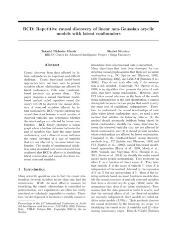
CausalityLatent confoudersTakashi Nicholas Maeda, Shohei ion1.00.00.5Recall0.000.250.50F-measure0.75Figure 3: Performance evaluation on causal graphs using simulated data: The vertical red lines indicate themedian values of the results. The evaluation of the latent confounders corresponds to the evaluation of bidirected arrows. The evaluation of causality corresponds to the evaluation of directed arrows.the number of all true arrows. F-measure is defined asF-measure 2 · precision · recall/(precision recall).The arguments of RCD, that is, αC (alpha level forPearson’s correlation), αI (alpha level for independence), αS (alpha level for the Shapiro-Wilk test), andn (maximum number of explanatory variables for multiple linear regression) were set as αC 0.01, αI 0.01, αS 0.01, and n 2.In regard to the types of edges, FCI, RFCI, and GFCIproduce partial ancestral graphs (PAGs) that includesix types of edges: (directed), (bi-directed), (partially directed), (nondirected), and (partially undirected). In the evaluation, we only used thedirected and bi-directed edges. PC, GES, LiNGAM,and RESIT produce causal graphs only with the directed edges; thus, we did not evaluate those methodsin terms of latent confounders.The box plots in Figure 3 display the results. Thevertical red lines indicate the median values. Notethat some median values are the same as the upperor lower quartiles. For example, the median and theupper quartile of the recalls of RCD in the results oflatent confounders are the same. It means that theresults between the median and the upper quartile arethe same. In regard to the evaluation of latent confounders, the precision, recall, and F-measure valuesare almost the same for RCD, FCI, RFCI, and GFCI,but the medians of precision, recall, and F-measurevalues of RCD are the highest among them. In regardto causality, RCD scores the highest medians of theprecision and F-measure values among all the methods, and the median of recall for RCD is the secondhighest next to RESIT.The results suggest that RCD does not greatly improve the performance metrics compared to the existing methods. However, there is no other method thathas the highest or the second highest performance foreach metric. FCI, RFCI, and GFCI perform as well asRCD in terms of finding the pairs of variables that areaffected by the same latent confounders, but they donot perform well in terms of the recall of causality. Inaddition, no other method performs well in terms ofboth precision and recall of causality. RCD can successfully find the pairs of variables that are affected bythe same latent confounders and identify the causal direction between variables that are not affected by thesame latent confounder.4.2Performance on real-world str

GES [Chickering, 2002], and LiNGAM [Shimizu et al., 2006]). They do not work effectively if this assump-tion is not satisfied. Conversely, FCI [Spirtes et al., 1999] is an algorithm that presents the pairs of vari-ables that have latent confounders. However, since FCI infers causal relations on the basis of the condi-