WIXLIB

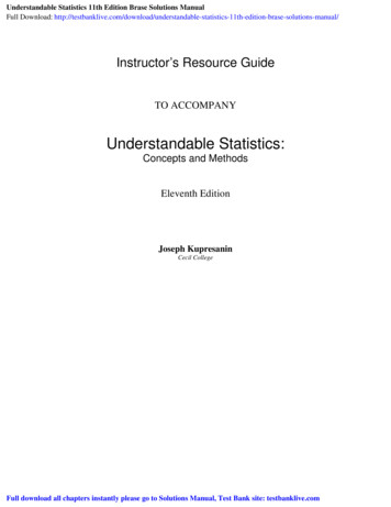
Teaching Tips for Each ChapterCHAPTER 1: GETTING STARTEDDouble-Blind Studies (Section 1.3)The double-blind method of data collection, mentioned at the end of Section 1.3, is an important part of standardresearch practice. A typical use is in testing new medications. Because the researcher does not know which patientsare receiving the experimental drug and which are receiving the established drug (or a placebo), the researcher isprevented from doing things subconsciously that might skew the results.If, for instance, the researcher communicates a more optimistic attitude to patients in the experimental group, thiscould influence how they respond to diagnostic questions or actually might influence the course of their illness. Andif the researcher wants the new drug to prove effective, this could subconsciously influence how he or she handlesinformation related to each patient’s case. All such factors are eliminated in double-blind testing.The following appears in the physician’s dosing instructions package insert for the prescription drug QUIXIN :In randomized, double-masked, multicenter controlled clinical trials where patients were dosed for5 days, QUIXIN demonstrated clinical cures in 79% of patients treated for bacterialconjunctivitis on the final study visit day (days 6–10).Note the phrase double-masked. Apparently, this is a synonym for double-blind. Since double-blind is used widelyin the medical literature and in clinical trials, why do you suppose that the company chose to use double-maskedinstead?Perhaps this will provide some insight: QUIXIN is a topical antibacterial solution for the treatment ofconjunctivitis; i.e., it is an antibacterial eye drop solution used to treat an inflammation of the conjunctiva, themucous membrane that lines the inner surface of the eyelid and the exposed surface of the eyeball. Perhaps, sinceQUIXIN is a treatment for eye problems, the manufacturer decided the word blind should not appear anywhere inthe discussion.Source: Package insert. QUIXIN is manufactured by Santen Oy, P.O. Box 33, FIN-33721 Tampere, Finland, andmarketed by Santen, Inc., Napa, CA 94558, under license from Daiichi Pharmaceutical Co., Ltd., Tokyo, Japan.CHAPTER 2: ORGANIZING DATAEmphasize when to use the various graphs discussed in this chapter: bar graphs when comparing data sets, circlegraphs for displaying how data are dispersed into several categories, time-series graphs to display how data changeover time, histograms or frequency polygons to display relative frequencies of grouped data, and stem-and-leafdisplays for displaying grouped data in a way that does not lose the detail of the original raw data.Drawing and Using Ogives (Section 2.1)The text describes how an ogive, which is a graph displaying a cumulative-frequency distribution, can beconstructed easily using a frequency table. However, a graph of the same basic sort can be constructed even morequickly than that. Simply arrange the data values in ascending order and then plot one point for each data value,where the x coordinate is the data value and the y coordinate starts at 1 for the first point and increases by 1 for eachsuccessive point. Finally, connect adjacent points with line segments. In the resulting graph, for any x, thecorresponding y value will be (roughly) the number of data values less than or equal to x.For example, here is the graph for the data set 64, 65, 68, 73, 74, 76, 81, 84, 85, 88, 92, 95, 95, and 99:6

This graph is not technically an ogive because the possibility of duplicate data values (such as 95 in this example)means that the graph will not necessarily be a function. But the graph can be used to get a quick fix on the generalshape of the cumulative distribution curve. And by implication, the graph can be used to get a quick idea of theshape of the frequency distribution, as illustrated below.Psuedo - Ogive Uniform DistributionUniform 20.480.640.800.960.01.120.20.40.60.81.0Psuedo - Ogive Normal DistributionNormal e pseudo-ogive obtained from the example data set suggests a uniform distribution on the interval 63–100 orthereabouts.CHAPTER 3: AVERAGES AND VARIATIONStudents should be instructed in the various ways that sets of numeric data can be represented by a single number.The concepts of this section illustrate for students the need for this kind of representation.7

The different ways this can be done are discussed in Section 3.1. The mean, median, and mode vary inappropriateness depending on the situation. In many cases of numeric data, the mean is the most appropriatemeasure of central tendency. If the mean is larger or smaller than most of the data values, however, then the medianmay be the number that best represents the data set. The median is most appropriate usually if the data set is annualsalaries, costs of houses, or any data set that contains one or a few very large or very small values. The mode wouldbe most appropriate if the population were the votes in an election or Nielsen television ratings, for example.Students should get acquainted with these concepts by calculating the mean, median, and mode for different datasets and then interpreting the meaning of each one and determining which measure of central tendency is the mostappropriate.The range, variance, and standard deviation can be presented to students as other numbers that aid in therepresentation of a data set in that they measure how data are dispersed. Students will begin to have a betterunderstanding of these measures of dispersion by calculating these numbers for given data sets and interpreting theirrespective meanings. These concepts of central tendency and dispersion also can be applied to grouped data, andstudents should become acquainted with interpreting these measures for given realistic situations in which data havebeen collected.Chebyshev’s theorem is important to discuss with students because it relates to the mean and standard deviation ofany data set.Finally, the mean, median, first and third quartiles, and range of a data set can be viewed easily in a box-andwhisker plot.CHAPTER 4: ELEMENTARY PROBABILITY THEORYWhat Is Probability? (Section 4.1)As the text describes, there are several methods for assigning a probability to an event. Probability based on intuitionis often called subjective probability. Thus understood, probability is a numerical measure of a person’s estimate ofthe likelihood of some event. Subjective probability is assumed to be reflected in a person’s decisions: The higher anevent’s probability, the more the person would be willing to bet on its occurring.Probability based on relative frequency is often called experimental probability because the relative frequency iscalculated from an observed history of experiment outcomes. But we are already using the word experiment in a waythat is neutral among the different treatments of probability—namely, as the name for the activity that producesvarious possible outcomes. So when we are talking about probability based on relative frequency, we will call thisobserved probability.Probability based on equally likely outcomes is often called theoretical probability because it is ultimately derivedfrom a theoretical model of the experiment’s structure. The experiment may be conducted only once, or not at all,and need not be repeatable.These three ways of treating probability are compatible and complementary. For a reasonable, well-informed person,the subjective probability of an event should match the theoretical probability, and the theoretical probability, inturn, predicts the observed probability as the experiment is repeated many times.Also, it should be noted that although in statistics probability is officially a property of events, it can be thought of asa property of statements as well. The probability of a statement equals the probability of the event that makes thestatement true.Probability and statistics are overlapping fields of study; if they weren’t, there would be no need for a chapter onprobability in a book on statistics. So the general statement in the text that probability deals with known populations,whereas statistics deals with unknown populations is necessarily a simplification. However, the statement doesexpress an important truth: If we confront an experiment we initially know absolutely nothing about, then we cancollect data but we cannot calculate probabilities. In other words, we can only calculate probabilities after we have8

formed some idea of, or acquaintance with, the experiment. To find the theoretical probability of an event, we haveto know how the experiment is set up. To find the observed probability, we have to have a record of previousoutcomes. And as reasonable people, we need some combination of those same two kinds of information to set oursubjective probability.This may seem obvious, but it has important implications for how we understand technical concepts encounteredlater in the course. There will be times when we would like to make a statement, say, about the mean of a populationand then give the probability that this statement is true—i.e., the probability that the event described by thestatement occurs (or has occurred). What we discover when we look closely, however, is that often this cannot bedone. Often we have to settle for some other conclusion instead. The Teaching Tips for Sections 7.1 and 8.1 describetwo instances of this problem.CHAPTER 5: THE BINOMIAL PROBABILITY DISTRIBUTION AND RELATEDTOPICSBinomial Probabilities (Section 5.2)Students should be able to show that pq p(1 – p) has its maximum value at p 0.5. There are at least three ways todemonstrate this: graphically, algebraically, and using calculus.Graphical methodRecall that 0 p 1. So, for q 1 – p, 0 q 1 and 0 pq 1. Plot y pq p(1 – p) using MINITAB, a graphingcalculator, or other technology. The graph is a parabola. Observe which value of p maximizes pq. (Many graphingcalculators can find the maximum value and where it occurs.)So pq has a maximum value of 0.25 when p 0.5.Algebraic methodFrom the definition of q, it follows that pq p(1 – p) p – p2 –p2 p 0. Recognize that this is a quadraticfunction of the form ax2 bx c, where p is used instead of x, and a –1, b 1, and c 0.The graph of a quadratic function is a parabola, and the general form of a parabola is y a(x – h)2 k. The parabolaopens up if a 0 and opens down if a 0 and has a vertex at (h, k). If the parabola opens up, it has its minimum at x h, and the minimum value of the function is y k. Similarly, if the parabola opens down, it has its maximum valueof y k, when x h.Using the method of completing the square, we can rewrite y ax2 bx c in the form y a(x – h)2 k to show thatbb2and k c . When a –1, b 1, and c 0, it follows that h 1/2 and k 1/4. So the value of p that2a4amaximizes pq is p 1/2, and then pq 1/4. This confirms the results of the graphical solution.h Calculus-based methodAdvanced Placement students probably have had (or are taking) calculus, including tests for local extrema. For afunction with continuous first and second derivatives, at an extremum, the first derivative equals 0, and the secondderivative is either positive (at a minimum) or negative (at a maximum).9

The first derivative of f(p) pq p(1 p) is given byd f ′( p )[ p (1 p )]dpd [ p 2 p]dp 2 p 1Solve f ′( p ) 0: 2 p 1 0p 12 1 Now find f ′′ : 2 df ′′( p ) [ f ′( p )]dpd ( 2 p 1)dp 2 1 So f ′′ 2. 2 1Since the second derivative is negative when the first derivative equals 0, f(p) has a maximum at p .2This result has implications for confidence intervals for p; see the Teaching Tips for Chapter 7.CHAPTER 6: NORMAL CURVES AND SAMPLING DISTRIBUTIONSEmphasize the differences between discrete and continuous random variables with examples of each.Emphasize how normal curves can be used to approximate the probabilities of both continuous and discrete randomvariables, and in the cases when the distribution of a data set can be approximated by a normal curve, such a curve isdefined by two quantities: the mean and standard deviation of the data. In such a case, the normal curve is definedby this equation:( )x µ 2y e 1 σ2σ 2πReview Chebyshev’s theorem from Chapter 3. Emphasize that this theorem implies that for any data set,at least 75% of the data lie within 2 standard deviations on each side of the mean, at least 88.9% of the data liewithin 3 standard deviations on each side of the mean, and at least 93.75% of the data lie within 4 standarddeviations on each side of the mean.In comparison, a data set that has a distribution that is symmetric and bell-shaped, or in particular, an approximatenormal distribution, is more restrictive in that1.2.3.Approximately 68% of the data values lie within 1 standard deviation on each side of the mean,Approximately 95% of the data values lie within 2 standard deviations on each side of the mean, andApproximately 99.7% of the data values lie within 3 standard deviations on each side of the mean.Remind students regularly that a z value equals the number of standard deviations from the mean for data values ofany distribution approximated by a normal curve.10

Emphasize the connection between the area under a normal curve and probability values of the random variable.That is, emphasize that the area under any normal curve equals 1 and that the percentage of area under the curvebetween given values of the random variable equals the probability that the random variable will be between thesevalues. The values in a z table are areas and probability values.Emphasize the differences between population parameters and sample statistics. Point out that when knowledge ofthe population is unavailable, then knowledge of a corresponding sample statistic must be used to make inferencesabout the population.Emphasize the main two facts derived from the central limit theorem:1.If x is a random variable with a normal distribution whose mean is μ and standard deviation is σ, then themeans of random samples for any fixed-size n taken from the x distribution is a random variable x that hasa normal distribution with mean μ and standard deviation σ n .2.If x is a random variable with any distribution whose mean is μ and standard deviation is σ, then the meanof random samples of a fixed-size n taken from the x distribution is a random variable x that has adistribution that approaches a normal distribution with mean μ and standard deviation σ n as n increaseswithout limit.Choosing sample sizes greater than 30 is an important point to emphasize in the situation mentioned in part 2 of thecentral limit theorem above. This commonly accepted convention ensures that the x distribution of part 2 will havean approximate normal distribution regardless of the distribution of the population from which these samples aredrawn.Emphasize that the central limit theorem allows us to infer facts about populations from sample means havingnormal distributions.Emphasize the conditions whereby a binomial probability distribution (discussed in Chapter 5) can be approximatedby a normal distribution: np 5 and n(1 – p) 5, where n is the number of trials and p is the probability of successin a single trial.When a normal distribution is used to approximate a discrete random variable (such as the random variable of abinomial probability experiment), the continuity correction is an important concept to emphasize to students. Adiscussion of this important adjustment can be a good opportunity to compare discrete and continuous randomvariables.Emphasize that facts about sampling distributions for proportions relating to binomial experiments can be inferred ifthe same conditions satisfied by a binomial experiment that can be approximated by a normal distribution aresatisfied: np 5 and n(1 – p) 5, where n is the number of trials and p is the probability of success in a single trial.Emphasize the difference in the continuity correction that must be taken into account in the sampling distribution forproportions and the continuity correction for a normal distribution used to approximate the probability distributionof the discrete random variable in a binomial probability experiment. That is, instead of subtracting 0.5 from the leftendpoint and adding 0.5 to the right endpoint of an interval involved in a normal distribution approximating abinomial probability distribution, 0.5/n must be subtracted from the left endpoint and 0.5/n must be added to theright endpoint of such an interval when a normal distribution is used to approximate a sampling distribution forproportions.CHAPTER 7: ESTIMATIONAs the text says, nontrivial probability statements involve variables, not constants. And if the mean of a populationis considered a constant, then the event that this mean falls in a certain range with known numerical bounds haseither probability 1 or probability 0.11

However, we might instead think of the population mean as itself a variable because, after all, the value of the meanis unknown initially. In other words, we may think of the population from which we are sampling as one of manypopulations—a population of populations, if you like. One of these populations has been randomly selected for us towork with, and we are trying to figure out which population it is or at least what its mean is.If we think of our sampling activity in this way, we can then think of the event “The mean lies between a and b” ashaving a nontrivial probability of being true. Can we now create a 90% confidence interval and then say that themean has a 90% probability of being in that interval? It might seem so, but in general, the answer is no. Even thougha procedure might have exactly a 90% success rate at creating confidence intervals that contain the mean, aconfidence interval created by such a procedure will not, in general, have exactly a 90% chance of containing themean.How is this possible? To understand this paradox, let us turn from mean finding to a simpler task: guessing the colorof a randomly drawn marble. Suppose that a sack contains some red marbles and some blue marbles. And supposethat we have a friend wh

Calculators and statistical computer software remove much of the computational burden from statistics. Many basic scientific calculators provide the mean and standard deviation. Calculators that support two-variable statistics provide the coefficients of the least-squares line, the value of the correlation coefficient, and the predicted value of