Transcription
5MCMC Using Hamiltonian DynamicsRadford M. Neal5.1IntroductionMarkov chain Monte Carlo (MCMC) originated with the classic paper of Metropolis et al.(1953), where it was used to simulate the distribution of states for a system of idealizedmolecules. Not long after, another approach to molecular simulation was introduced (Alderand Wainwright, 1959), in which the motion of the molecules was deterministic, followingNewton’s laws of motion, which have an elegant formalization as Hamiltonian dynamics. Forfinding the properties of bulk materials, these approaches are asymptotically equivalent,since even in a deterministic simulation, each local region of the material experienceseffectively random influences from distant regions. Despite the large overlap in their application areas, the MCMC and molecular dynamics approaches have continued to coexist inthe following decades (see Frenkel and Smit, 1996).In 1987, a landmark paper by Duane, Kennedy, Pendleton, and Roweth united theMCMC and molecular dynamics approaches. They called their method “hybrid MonteCarlo,” which abbreviates to “HMC,” but the phrase “Hamiltonian Monte Carlo,” retaining the abbreviation, is more specific and descriptive, and I will use it here. Duane et al.applied HMC not to molecular simulation, but to lattice field theory simulations of quantum chromodynamics. Statistical applications of HMC began with my use of it for neuralnetwork models (Neal, 1996a). I also provided a statistically-oriented tutorial on HMC in areview of MCMC methods (Neal, 1993, Chapter 5). There have been other applicationsof HMC to statistical problems (e.g. Ishwaran, 1999; Schmidt, 2009) and statisticallyoriented reviews (e.g. Liu, 2001, Chapter 9), but HMC still seems to be underappreciatedby statisticians, and perhaps also by physicists outside the lattice field theory community.This review begins by describing Hamiltonian dynamics. Despite terminology that maybe unfamiliar outside physics, the features of Hamiltonian dynamics that are needed forHMC are elementary. The differential equations of Hamiltonian dynamics must be discretized for computer implementation. The “leapfrog” scheme that is typically used isquite simple.Following this introduction to Hamiltonian dynamics, I describe how to use it to construct an MCMC method. The first step is to define a Hamiltonian function in terms of theprobability distribution we wish to sample from. In addition to the variables we are interested in (the “position” variables), we must introduce auxiliary “momentum” variables,which typically have independent Gaussian distributions. The HMC method alternatessimple updates for these momentum variables with Metropolis updates in which a newstate is proposed by computing a trajectory according to Hamiltonian dynamics, implemented with the leapfrog method. A state proposed in this way can be distant from the113
114Handbook of Markov Chain Monte Carlocurrent state but nevertheless have a high probability of acceptance. This bypasses the slowexploration of the state space that occurs when Metropolis updates are done using a simplerandom-walk proposal distribution. (An alternative way of avoiding random walks is to useshort trajectories but only partially replace the momentum variables between trajectories,so that successive trajectories tend to move in the same direction.)After presenting the basic HMC method, I discuss practical issues of tuning the leapfrogstepsize and number of leapfrog steps, as well as theoretical results on the scaling of HMCwith dimensionality. I then present a number of variations on HMC. The acceptance ratefor HMC can be increased for many problems by looking at “windows” of states at thebeginning and end of the trajectory. For many statistical problems, approximate computation of trajectories (e.g. using subsets of the data) may be beneficial. Tuning of HMC canbe made easier using a “short-cut” in which trajectories computed with a bad choice ofstepsize take little computation time. Finally, “tempering” methods may be useful whenmultiple isolated modes exist.5.2Hamiltonian DynamicsHamiltonian dynamics has a physical interpretation that can provide useful intuitions.In two dimensions, we can visualize the dynamics as that of a frictionless puck that slidesover a surface of varying height. The state of this system consists of the position of the puck,given by a two-dimensional vector q, and the momentum of the puck (its mass times itsvelocity), given by a two-dimensional vector p. The potential energy, U(q), of the puck isproportional to the height of the surface at its current position, and its kinetic energy, K(p),is equal to p 2 /(2m), where m is the mass of the puck. On a level part of the surface, thepuck moves at a constant velocity, equal to p/m. If it encounters a rising slope, the puck’smomentum allows it to continue, with its kinetic energy decreasing and its potential energyincreasing, until the kinetic energy (and hence p) is zero, at which point it will slide backdown (with kinetic energy increasing and potential energy decreasing).In nonphysical MCMC applications of Hamiltonian dynamics, the position will correspond to the variables of interest. The potential energy will be minus the log of theprobability density for these variables. Momentum variables, one for each position variable,will be introduced artificially.These interpretations may help motivate the exposition below, but if you find otherwise,the dynamics can also be understood as simply resulting from a certain set of differentialequations.5.2.1Hamilton’s EquationsHamiltonian dynamics operates on a d-dimensional position vector, q, and a d-dimensionalmomentum vector, p, so that the full state space has 2d dimensions. The system is describedby a function of q and p known as the Hamiltonian, H(q, p).5.2.1.1Equations of MotionThe partial derivatives of the Hamiltonian determine how q and p change over time, t,according to Hamilton’s equations:
115MCMC Using Hamiltonian Dynamicsdqi H ,dt pi(5.1)dpi H ,dt qi(5.2)for i 1, . . ., d. For any time interval of duration s, these equations define a mapping, Ts ,from the state at any time t to the state at time t s. (Here, H, and hence Ts , are assumed tonot depend on t.)Alternatively, we can combine the vectors q and p into the vector z (q, p) with 2ddimensions, and write Hamilton’s equations asdz J H(z),dtwhere H is the gradient of H (i.e. [ H]k H/ zk ), and0J 0d d Id dId d0d d1(5.3)is a 2d 2d matrix whose quadrants are defined above in terms of identity and zero matrices.5.2.1.2Potential and Kinetic EnergyFor HMC we usually use Hamiltonian functions that can be written asH(q, p) U(q) K(p).(5.4)Here U(q) is called the potential energy, and will be defined to be minus the log probabilitydensity of the distribution for q that we wish to sample, plus any constant that is convenient.K(p) is called the kinetic energy, and is usually defined asK(p) pT M 1 p/2.(5.5)Here M is a symmetric, positive-definite “mass matrix,” which is typically diagonal, andis often a scalar multiple of the identity matrix. This form for K(p) corresponds to minusthe log probability density (plus a constant) of the zero-mean Gaussian distribution withcovariance matrix M.With these forms for H and K, Hamilton’s equations 5.1 and 5.2 can be written as follows,for i 1, . . ., d:dqi [M 1 p]i ,dt Udpi .dt qi(5.6)(5.7)
116Handbook of Markov Chain Monte Carlo5.2.1.3 A One-Dimensional ExampleConsider a simple example in one dimension (for which q and p are scalars and will bewritten without subscripts), in which the Hamiltonian is defined as follows:H(q, p) U(q) K(p),U(q) q2,2K(p) p2.2(5.8)As we will see later in Section 5.3.1, this corresponds to a Gaussian distribution for q withmean zero and variance one. The dynamics resulting from this Hamiltonian (followingEquations 5.6 and 5.7) isdqdp p, q.dtdtSolutions have the following form, for some constants r and a:q(t) r cos(a t),p(t) r sin(a t).(5.9)Hence, the mapping Ts is a rotation by s radians clockwise around the origin in the (q, p)plane. In higher dimensions, Hamiltonian dynamics generally does not have such a simpleperiodic form, but this example does illustrate some important properties that we will lookat next.5.2.2Properties of Hamiltonian DynamicsSeveral properties of Hamiltonian dynamics are crucial to its use in constructing MCMCupdates.5.2.2.1ReversibilityFirst, Hamiltonian dynamics is reversible—the mapping Ts from the state at time t, (q(t), p(t)),to the state at time t s, (q(t s), p(t s)), is one-to-one, and hence has an inverse, T s .This inverse mapping is obtained by simply negating the time derivatives in Equations5.1 and 5.2. When the Hamiltonian has the form in Equation 5.4, and K(p) K( p), as inthe quadratic form for the kinetic energy of Equation 5.5, the inverse mapping can also beobtained by negating p, applying Ts , and then negating p again.In the simple one-dimensional example of Equation 5.8, T s is just a counterclockwiserotation by s radians, undoing the clockwise rotation of Ts .The reversibility of Hamiltonian dynamics is important for showing that MCMC updatesthat use the dynamics leave the desired distribution invariant, since this is most easily proved by showing reversibility of the Markov chain transitions, which requiresreversibility of the dynamics used to propose a state.5.2.2.2Conservation of the HamiltonianA second property of the dynamics is that it keeps the Hamiltonian invariant (i.e. conserved).This is easily seen from Equations 5.1 and 5.2 as follows:1 1d 0d 0 dHdqi H H Hdpi H H H 0. dtdt qidt pi pi qi qi pii 1i 1(5.10)
117MCMC Using Hamiltonian DynamicsWith the Hamiltonian of Equation 5.8, the value of the Hamiltonian is half the squareddistance from the origin, and the solutions (Equation 5.9) stay at a constant distance fromthe origin, keeping H constant.For Metropolis updates using a proposal found by Hamiltonian dynamics, which formpart of the HMC method, the acceptance probability is one if H is kept invariant. We willsee later, however, that in practice we can only make H approximately invariant, and hencewe will not quite be able to achieve this.5.2.2.3 Volume PreservationA third fundamental property of Hamiltonian dynamics is that it preserves volume in (q, p)space (a result known as Liouville’s theorem). If we apply the mapping Ts to the pointsin some region R of (q, p) space, with volume V, the image of R under Ts will also havevolume V.With the Hamiltonian of Equation 5.8, the solutions (Equation 5.9) are rotations, whichobviously do not change the volume. Such rotations also do not change the shape of aregion, but this is not so in general—Hamiltonian dynamics might stretch a region in onedirection, as long as the region is squashed in some other direction so as to preserve volume.The significance of volume preservation for MCMC is that we need not account for anychange in volume in the acceptance probability for Metropolis updates. If we proposednew states using some arbitrary, non-Hamiltonian, dynamics, we would need to computethe determinant of the Jacobian matrix for the mapping the dynamics defines, which mightwell be infeasible.The preservation of volume by Hamiltonian dynamics can be proved in several ways.One is to note that the divergence of the vector field defined by Equations 5.1 and 5.2 iszero, which can be seen as follows:)*1 1 d 0d 0d 2H dqi H dpi H 2H 0. qi dt pi dt qi pi pi qi qi pi pi qii 1i 1i 1A vector field with zero divergence can be shown to preserve volume (Arnold, 1989).Here, I will show informally that Hamiltonian dynamics preserves volume more directly,without presuming this property of the divergence. I will, however, take as given thatvolume preservation is equivalent to the determinant of the Jacobian matrix of Ts havingabsolute value one, which is related to the well-known role of this determinant in regardto the effect of transformations on definite integrals and on probability density functions.The 2d 2d Jacobian matrix of Ts , seen as a mapping of z (q, p), will be written as Bs . Ingeneral, Bs will depend on the values of q and p before the mapping. When Bs is diagonal,it is easy to see that the absolute values of its diagonal elements are the factors by whichTs stretches or compresses a region in each dimension, so that the product of these factors,which is equal to the absolute value of det(Bs ), is the factor by which the volume of theregion changes. I will not prove the general result here, but note that if we were to (say)rotate the coordinate system used, Bs would no longer be diagonal, but the determinantof Bs is invariant to such transformations, and so would still give the factor by which thevolume changes.Let us first consider volume preservation for Hamiltonian dynamics in one dimension(i.e. with d 1), for which we can drop the subscripts on p and q. We can approximate Tδ
118Handbook of Markov Chain Monte Carlofor δ near zero as follows:Tδ (q, p) ) *q) δpdq/dtdp/dt* terms of order δ2 or higher.Taking the time derivatives from Equations 5.1 and 5.2, the Jacobian matrix can be written as 2H 1 δ q p Bδ 2H δ 2 qδ 2H p21 δ terms of order δ2 or higher.2 H (5.11) p qWe can then write the determinant of this matrix asdet(Bδ ) 1 δ 2H 2H δ terms of order δ2 or higher q p p q 1 terms of order δ2 or higher.Since log(1 x) x for x near zero, log det(Bδ ) is zero, except perhaps for terms of orderδ2 or higher (though we will see later that it is exactly zero). Now consider log det(Bs ) forsome time interval s that is not close to zero. Setting δ s/n, for some integer n, we canwrite Ts as the composition of Tδ applied n times (from n points along the trajectory), sodet(Bs ) is the n-fold product of det(Bδ ) evaluated at these points. We then find thatlog det(Bs ) n log det(Bδ )i 1 n # terms of order 1/n2 or smaller(5.12)i 1 terms of order 1/n or smaller.Note that the value of Bδ in the sum in Equation 5.12 might perhaps vary with i, sincethe values of q and p vary along the trajectory that produces Ts . However, assuming thattrajectories are not singular, the variation in Bδ must be bounded along any particulartrajectory. Taking the limit as n , we conclude that log det(Bs ) 0, so det(Bs ) 1, andhence Ts preserves volume.When d 1, the same argument applies. The Jacobian matrix will now have the followingform (compare Equation 5.11), where each entry shown below is a d d submatrix, withrows indexed by i and columns by j: * 2H I δ qj pi Bδ )* 2 δ H qj qi)) 2Hδ pj pi* 2 )* terms of order δ or higher. 2H I δ pj qi
119MCMC Using Hamiltonian DynamicsAs for d 1, the determinant of this matrix will be one plus terms of order δ2 or higher,since all the terms of order δ cancel. The remainder of the argument above then applieswithout change.5.2.2.4SymplecticnessVolume preservation is also a consequence of Hamiltonian dynamics being symplectic. Letting z (q, p), and defining J as in Equation 5.3, the symplecticness condition is that theJacobian matrix, Bs , of the mapping Ts satisfiesBTs J 1 Bs J 1 .This implies volume conservation, since det(BTs ) det( J 1 ) det(Bs ) det( J 1 ) implies thatdet(Bs )2 is one. When d 1, the symplecticness condition is stronger than volume preservation. Hamiltonian dynamics and the symplecticness condition can be generalized to whereJ is any matrix for which J T J and det( J) 0.Crucially, reversibility, preservation of volume, and symplecticness can be maintainedexactly even when, as is necessary in practice, Hamiltonian dynamics is approximated, aswe will see next.5.2.3Discretizing Hamilton’s Equations—The Leapfrog MethodFor computer implementation, Hamilton’s equations must be approximated by discretizingtime, using some small stepsize, ε. Starting with the state at time zero, we iteratively compute(approximately) the state at times ε, 2ε, 3ε, etc.In discussing how to do this, I will assume that the Hamiltonian has the form H(q, p) U(q) K(p), as in Equation 5.4. Although the methods below can be applied with any formfor the kinetic energy, I assume for simplicity that K(p) pT M 1 p/2, as in Equation 5.5, andfurthermore that M is diagonal, with diagonal elements m1 , . . . , md , so thatd p2i.K(p) 2mi(5.13)i 15.2.3.1Euler’s MethodPerhaps the best-known way to approximate the solution to a system of differential equations is Euler’s method. For Hamilton’s equations, this method performs the followingsteps, for each component of position and momentum, indexed by i 1, . . ., d:pi (t ε) pi (t) εdpi U(t) pi (t) ε(q(t)),dt qi(5.14)qi (t ε) qi (t) εdqipi (t)(t) qi (t) ε.dtmi(5.15)The time derivatives in Equations 5.14 and 5.15 are from the form of Hamilton’s equations given by Equations 5.6 and 5.7. If we start at t 0 with given values for qi (0) andpi (0), we can iterate the steps above to get a trajectory of position and momentum values
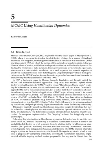
120Handbook of Markov Chain Monte Carloat times ε, 2ε, 3ε, . . . , and hence find (approximate) values for q(τ) and p(τ) after τ/ε steps(assuming τ/ε is an integer).Figure 5.1a shows the result of using Euler’s method to approximate the dynamics definedby the Hamiltonian of Equation 5.8, starting from q(0) 0 and p(0) 1, and using a stepsizeof ε 0.3 for 20 steps (i.e. to τ 0.3 20 6). The results are not good—Euler’s methodproduces a trajectory that diverges to infinity, but the true trajectory is a circle. Using asmaller value of ε, and correspondingly more steps, produces a more accurate result atτ 6, but although the divergence to infinity is slower, it is not eliminated.Modified Euler’s method, stepsize 0.3221100 1 1 2 2 2(c) 10Position (q)1 22Leapfrog method, stepsize 0.3(d)2110 1 2 2 10Position (q)120Position (q)120 1 2 1Leapfrog method, stepsize 1.22Momentum ( p)Momentum ( p)(b)Euler’s method, stepsize 0.3Momentum ( p)Momentum ( p)(a) 2 10Position (q)12FIGURE 5.1Results using three methods for approximating Hamiltonian dynamics, when H(q, p) q2 /2 p2 /2. The initialstate was q 0, p 1. The stepsize was ε 0.3 for (a), (b), and (c), and ε 1.2 for (d). Twenty steps of the simulatedtrajectory are shown for each method, along with the true trajectory (in gray).
121MCMC Using Hamiltonian Dynamics5.2.3.2 A Modification of Euler’s MethodMuch better results can be obtained by slightly modifying Euler’s method, as follows:pi (t ε) pi (t) ε U(q(t)), qi(5.16)qi (t ε) qi (t) εpi (t ε).mi(5.17)We simply use the new value for the momentum variables, pi , when computing the newvalue for the position variables, qi . A method with similar performance can be obtained byinstead updating the qi first and using their new values to update the pi .Figure 5.1b shows the results using this modification of Euler’s method with ε 0.3.Though not perfect, the trajectory it produces is much closer to the true trajectory thanthat obtained using Euler’s method, with no tendency to diverge to infinity. This betterperformance is related to the modified method’s exact preservation of volume, which helpsavoid divergence to infinity or spiraling into the origin, since these would typically involvethe volume expanding to infinity or contracting to zero.To see that this modification of Euler’s method preserves volume exactly despite thefinite discretization of time, note that both the transformation from (q(t), p(t)) to (q(t),p(t ε)) via Equation 5.16 and the transformation from (q(t), p(t ε)) to (q(t ε), p(t ε))via Equation 5.17 are “shear” transformations, in which only some of the variables change(either the pi or the qi ), by amounts that depend only on the variables that do not change.Any shear transformation will preserve volume, since its Jacobian matrix will have determinant one (as the only nonzero term in the determinant will be the product of diagonalelements, which will all be one).5.2.3.3 The Leapfrog MethodEven better results can be obtained with the leapfrog method, which works as follows:pi (t ε/2) pi (t) (ε/2)qi (t ε) qi (t) ε U(q(t)), qipi (t ε/2),mipi (t ε) pi (t ε/2) (ε/2) U(q(t ε)). qi(5.18)(5.19)(5.20)We start with a half step for the momentum variables, then do a full step for the positionvariables, using the new values of the momentum variables, and finally do another half stepfor the momentum variables, using the new values for the position variables. An analogousscheme can be used with any kinetic energy function, with K/ pi replacing pi /mi above.When we apply Equations 5.18 through 5.20 a second time to go from time t ε to t 2ε,we can combine the last half step of the first update, from pi (t ε/2) to pi (t ε), with thefirst half step of the second update, from pi (t ε) to pi (t ε ε/2). The leapfrog methodthen looks very similar to the modification of Euler’s method in Equations 5.17 and 5.16,except that leapfrog performs half steps for momentum at the very beginning and very endof the trajectory, and the time labels of the momentum values computed are shifted by ε/2.
122Handbook of Markov Chain Monte CarloThe leapfrog method preserves volume exactly, since Equations 5.18 through 5.20 areshear transformations. Due to its symmetry, it is also reversible by simply negating p,applying the same number of steps again, and then negating p again.Figure 5.1c shows the results using the leapfrog method with a stepsize of ε 0.3, whichare indistinguishable from the true trajectory, at the scale of this plot. In Figure 5.1d, theresults of using the leapfrog method with ε 1.2 are shown (still with 20 steps, so almostfour cycles are seen, rather than almost one). With this larger stepsize, the approximationerror is clearly visible, but the trajectory still remains stable (and will stay stable indefinitely).Only when the stepsize approaches ε 2 do the trajectories become unstable.5.2.3.4Local and Global Error of Discretization MethodsI will briefly discuss how the error from discretizing the dynamics behaves in the limit asthe stepsize, ε, goes to zero; Leimkuhler and Reich (2004) provide a much more detaileddiscussion. For useful methods, the error goes to zero as ε goes to zero, so that any upper limiton the error will apply (apart from a usually unknown constant factor) to any differentiablefunction of state—for example, if the error for (q, p) is no more than order ε2 , the error forH(q, p) will also be no more than order ε2 .The local error is the error after one step, that moves from time t to time t ε. The globalerror is the error after simulating for some fixed time interval, s, which will require s/εsteps. If the local error is order εp , the global error will be order εp 1 —the local errors oforder εp accumulate over the s/ε steps to give an error of order εp 1 . If we instead fix εand consider increasing the time, s, for which the trajectory is simulated, the error can ingeneral increase exponentially with s. Interestingly, however, this is often not what happens when simulating Hamiltonian dynamics with a symplectic method, as can be seen inFigure 5.1.The Euler method and its modification above have order ε2 local error and order ε globalerror. The leapfrog method has order ε3 local error and order ε2 global error. As shown byLeimkuhler and Reich (2004, Section 4.3.3), this difference is a consequence of leapfrog beingreversible, since any reversible method must have global error that is of even order in ε.5.3MCMC from Hamiltonian DynamicsUsing Hamiltonian dynamics to sample from a distribution requires translating the densityfunction for this distribution to a potential energy function and introducing “momentum”variables to go with the original variables of interest (now seen as “position” variables). Wecan then simulate a Markov chain in which each iteration resamples the momentum andthen does a Metropolis update with a proposal found using Hamiltonian dynamics.5.3.1Probability and the Hamiltonian: Canonical DistributionsThe distribution we wish to sample can be related to a potential energy function via theconcept of a canonical distribution from statistical mechanics. Given some energy function,E(x), for the state, x, of some physical system, the canonical distribution over states hasprobability or probability density function E(x)1exp.(5.21)P(x) ZT
MCMC Using Hamiltonian Dynamics123Here, T is the temperature of the system, and Z is the normalizing constant needed forthis function to sum or integrate to one. Viewing this the opposite way, if we are interestedin some distribution with density function P(x), we can obtain it as a canonical distribution with T 1 by setting E(x) log P(x) log Z, where Z is any convenient positiveconstant.The Hamiltonian is an energy function for the joint state of “position,” q, and “momentum,” p, and so defines a joint distribution for them as follows: 1 H(q, p)P(q, p) exp.ZTNote that the invariance of H under Hamiltonian dynamics means that a Hamiltoniantrajectory will (if simulated exactly) move within a hypersurface of constant probabilitydensity.If H(q, p) U(q) K(p), the joint density is 1 U(q) K(p)P(q, p) expexp,ZTT(5.22)and we see that q and p are independent, and each have canonical distributions, with energyfunctions U(q) and K(p). We will use q to represent the variables of interest, and introducep just to allow Hamiltonian dynamics to operate.In Bayesian statistics, the posterior distribution for the model parameters is the usualfocus of interest, and hence these parameters will take the role of the position, q. We canexpress the posterior distribution as a canonical distribution (with T 1) using a potentialenergy function defined asU(q) log π(q)L(q D) ,where π(q) is the prior density, and L(q D) is the likelihood function given data D.5.3.2 The Hamiltonian Monte Carlo AlgorithmWe now have the background needed to present the Hamiltonian Monte Carlo algorithm.HMC can be used to sample only from continuous distributions on Rd for which the density function can be evaluated (perhaps up to an unknown normalizing constant). For themoment, I will also assume that the density is nonzero everywhere (but this is relaxed inSection 5.5.1). We must also be able to compute the partial derivatives of the log of thedensity function. These derivatives must therefore exist, except perhaps on a set of pointswith probability zero, for which some arbitrary value could be returned.HMC samples from the canonical distribution for q and p defined by Equation 5.22, inwhich q has the distribution of interest, as specified using the potential energy functionU(q). We can choose the distribution of the momentum variables, p, which are independentof q, as we wish, specifying the distribution via the kinetic energy function, K(p). Currentpractice with HMC is to use a quadratic kinetic energy, as in Equation 5.5, which leadsp to have a zero-mean multivariate Gaussian distribution. Most often, the components of Note to physicists: I assume here that temperature is measured in units that make Boltzmann’s constant unity.
124Handbook of Markov Chain Monte Carlop are specified to be independent, with component i having variance mi . The kinetic energyfunction producing this distribution (setting T 1) isK(p) d p2i.2mi(5.23)i 1We will see in Section 5.4 how the choice for the mi affects performance.5.3.2.1 The Two Steps of the HMC AlgorithmEach iteration of the HMC algorithm has two steps. The first changes only the momentum;the second may change both position and momentum. Both steps leave the canonical jointdistribution of (q, p) invariant, and hence their combination also leaves this distributioninvariant.In the first step, new values for the momentum variables are randomly drawn from theirGaussian distribution, independently of the current values of the position variables. For thekinetic energy of Equation 5.23, the d momentum variables are independent, with pi havingmean zero and variance mi . Since q is not changed, and p is drawn from its correct conditionaldistribution given q (the same as its marginal distribution, due to independence), this stepobviously leaves the canonical joint distribution invariant.In the second step, a Metropolis update is performed, using Hamiltonian dynamics topropose a new state. Starting with the current state, (q, p), Hamiltonian dynamics is simulated for L steps using the leapfrog method (or some other reversible method that preservesvolume), with a stepsize of ε. Here, L and ε are parameters of the algorithm, which need tobe tuned to obtain good performance (as discussed below in Section 5.4.2). The momentumvariables at the end of this L-step trajectory are then negated, giving a proposed state (q , p ).This proposed state is accepted as the next state of the Markov chain with probabilitymin 1, exp( H(q , p ) H(q, p)) min 1, exp( U(q ) U(q) K(p ) K(p)) .If the proposed state is not accepted (i.e. it is rejected), the next state is the same as the currentstate (and is counted again when estimating the expectation of some function of state byits average over states of the Markov chain). The negation of the momentum variables atthe end of the trajectory makes the Metropolis proposal symmetrical, as needed for theacceptance probability above to be valid. This negation need not be done in practice, sinceK(p) K( p), and the momentum will be replaced before it is used again, in the first stepof the next iteration. (This assumes that these HMC updates are the only ones performed.)If we look at HMC as sampling from the joint distribution of q and p, the Metropolis stepusing a proposal found by Hamiltonian dynamics leaves the probability density for (q, p)unchanged or almost unchanged. Movement to (q, p) points with a different probabilitydensity is accomplished only by t
MCMC Using Hamiltonian Dynamics 115 dqi dt H pi, (5.1) dpi dt H qi, (5.2) for i 1,.,d.For any time interval of duration s, these equations define a mapping, Ts, from the state at any time t to the state at time t s. (Here, H, and hence Ts, are assumed to not depend on t.) Alternatively, we can combine the vectors q and p into the vector z (q,p) with 2d .