Transcription
J. R. Statist. Soc. B (2005)67, Part 2, pp. 301–320Regularization and variable selection via theelastic netHui Zou and Trevor HastieStanford University, USA[Received December 2003. Final revision September 2004]Summary. We propose the elastic net, a new regularization and variable selection method. Realworld data and a simulation study show that the elastic net often outperforms the lasso, whileenjoying a similar sparsity of representation. In addition, the elastic net encourages a groupingeffect, where strongly correlated predictors tend to be in or out of the model together. The elasticnet is particularly useful when the number of predictors (p) is much bigger than the number ofobservations (n). By contrast, the lasso is not a very satisfactory variable selection method in thep n case. An algorithm called LARS-EN is proposed for computing elastic net regularizationpaths efficiently, much like algorithm LARS does for the lasso.Keywords: Grouping effect; LARS algorithm; Lasso; Penalization; p n problem; Variableselection1.Introduction and motivationWe consider the usual linear regression model: given p predictors x1 , . . . , xp , the response y ispredicted byŷ β̂ 0 x1 β̂ 1 . . . xp β̂ p :.1/A model fitting procedure produces the vector of coefficients β̂ .β̂ 0 , . . . , β̂ p /. For example, theordinary least squares (OLS) estimates are obtained by minimizing the residual sum of squares.The criteria for evaluating the quality of a model will differ according to the circumstances.Typically the following two aspects are important:(a) accuracy of prediction on future data—it is difficult to defend a model that predictspoorly;(b) interpretation of the model—scientists prefer a simpler model because it puts more lighton the relationship between the response and covariates. Parsimony is especially an important issue when the number of predictors is large.It is well known that OLS often does poorly in both prediction and interpretation. Penalization techniques have been proposed to improve OLS. For example, ridge regression (Hoerl andKennard, 1988) minimizes the residual sum of squares subject to a bound on the L2 -norm of thecoefficients. As a continuous shrinkage method, ridge regression achieves its better predictionperformance through a bias–variance trade-off. However, ridge regression cannot produce aparsimonious model, for it always keeps all the predictors in the model. Best subset selection inAddress for correspondence: Trevor Hastie, Department of Statistics, Stanford University, Stanford, CA 94305,USA.E-mail: hastie@stanford.edu 2005 Royal Statistical Society1369–7412/05/67301
302H. Zou and T. Hastiecontrast produces a sparse model, but it is extremely variable because of its inherent discreteness,as addressed by Breiman (1996).A promising technique called the lasso was proposed by Tibshirani (1996). The lasso is apenalized least squares method imposing an L1 -penalty on the regression coefficients. Owingto the nature of the L1 -penalty, the lasso does both continuous shrinkage and automatic variable selection simultaneously. Tibshirani (1996) and Fu (1998) compared the prediction performance of the lasso, ridge and bridge regression (Frank and Friedman, 1993) and foundthat none of them uniformly dominates the other two. However, as variable selection becomesincreasingly important in modern data analysis, the lasso is much more appealing owing to itssparse representation.Although the lasso has shown success in many situations, it has some limitations. Considerthe following three scenarios.(a) In the p n case, the lasso selects at most n variables before it saturates, because of thenature of the convex optimization problem. This seems to be a limiting feature for avariable selection method. Moreover, the lasso is not well defined unless the bound onthe L1 -norm of the coefficients is smaller than a certain value.(b) If there is a group of variables among which the pairwise correlations are very high, thenthe lasso tends to select only one variable from the group and does not care which one isselected. See Section 2.3.(c) For usual n p situations, if there are high correlations between predictors, it has beenempirically observed that the prediction performance of the lasso is dominated by ridgeregression (Tibshirani, 1996).Scenarios (a) and (b) make the lasso an inappropriate variable selection method in some situations. We illustrate our points by considering the gene selection problem in microarray dataanalysis. A typical microarray data set has many thousands of predictors (genes) and oftenfewer than 100 samples. For those genes sharing the same biological ‘pathway’, the correlationsbetween them can be high (Segal and Conklin, 2003). We think of those genes as forming agroup. The ideal gene selection method should be able to do two things: eliminate the trivialgenes and automatically include whole groups into the model once one gene among them isselected (‘grouped selection’). For this kind of p n and grouped variables situation, the lassois not the ideal method, because it can only select at most n variables out of p candidates (Efronet al., 2004), and it lacks the ability to reveal the grouping information. As for prediction performance, scenario (c) is not rare in regression problems. So it is possible to strengthen furtherthe prediction power of the lasso.Our goal is to find a new method that works as well as the lasso whenever the lasso does thebest, and can fix the problems that were highlighted above, i.e. it should mimic the ideal variableselection method in scenarios (a) and (b), especially with microarray data, and it should deliverbetter prediction performance than the lasso in scenario (c).In this paper we propose a new regularization technique which we call the elastic net. Similarto the lasso, the elastic net simultaneously does automatic variable selection and continuousshrinkage, and it can select groups of correlated variables. It is like a stretchable fishing net thatretains ‘all the big fish’. Simulation studies and real data examples show that the elastic net oftenoutperforms the lasso in terms of prediction accuracy.In Section 2 we define the naı̈ve elastic net, which is a penalized least squares method using anovel elastic net penalty. We discuss the grouping effect that is caused by the elastic net penalty.In Section 3, we show that this naı̈ve procedure tends to overshrink in regression problems. Wethen introduce the elastic net, which corrects this problem. An efficient algorithm LARS-EN is
Elastic Net303proposed for computing the entire elastic net regularization paths with the computational effortof a single OLS fit. Prostate cancer data are used to illustrate our methodology in Section 4,and simulation results comparing the lasso and the elastic net are presented in Section 5.Section 6 shows an application of the elastic net to classification and gene selection in a leukaemia microarray problem.2.Naı̈ve elastic net2.1. DefinitionSuppose that the data set has n observations with p predictors. Let y .y1 , . . . , yn /T be theresponse and X .x1 . . . xp / be the model matrix, where xj .x1j , . . . , xnj /T , j 1, . . . , p, arethe predictors. After a location and scale transformation, we can assume that the response iscentred and the predictors are standardized,n i 1yi 0,n i 1xij 0andn i 12xij 1,for j 1, 2, . . . , p:.2/For any fixed non-negative λ1 and λ2 , we define the naı̈ve elastic net criterionL.λ1 , λ2 , β/ y Xβ 2 λ2 β 2 λ1 β 1 ,.3/where β 2 β 1 p j 1p j 1βj2 , βj :The naı̈ve elastic net estimator β̂ is the minimizer of equation (3):β̂ arg min{L.λ1 , λ2 , β/}:β.4/This procedure can be viewed as a penalized least squares method. Let α λ2 .λ1 λ2 /; thensolving β̂ in equation (3) is equivalent to the optimization problemβ̂ arg min y Xβ 2 ,βsubject to .1 α/ β 1 α β 2 t for some t:.5/We call the function .1 α/ β 1 α β 2 the elastic net penalty, which is a convex combinationof the lasso and ridge penalty. When α 1, the naı̈ve elastic net becomes simple ridge regression.In this paper, we consider only α 1. For all α [0, 1/, the elastic net penalty function is singular(without first derivative) at 0 and it is strictly convex for all α 0, thus having the characteristicsof both the lasso and ridge regression. Note that the lasso penalty (α 0) is convex but notstrictly convex. These arguments can be seen clearly from Fig. 1.2.2. SolutionWe now develop a method to solve the naı̈ve elastic net problem efficiently. It turns out thatminimizing equation (3) is equivalent to a lasso-type optimization problem. This fact impliesthat the naı̈ve elastic net also enjoys the computational advantage of the lasso.
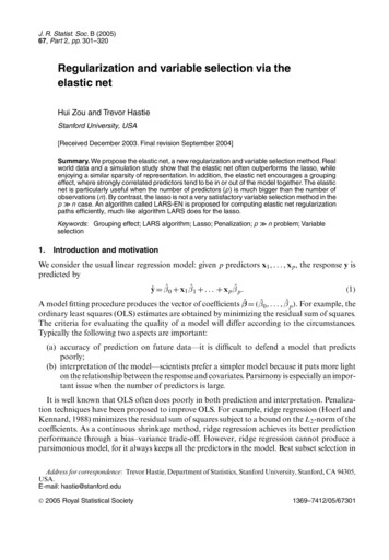
304H. Zou and T. Hastieβ2β1Fig. 1. Two-dimensional contour plots (level 1) ( - - -, shape of the ridge penalty; - - - - - - -, contour of thelasso penalty;, contour of the elastic net penalty with α D 0:5): we see that singularities at the verticesand the edges are strictly convex; the strength of convexity varies with αLemma 1. Given data set .y, X/ and .λ1 , λ2 /, define an artificial data set .yÅ , XÅ / by yÅ 1 2 XÅX.n p/ p .1 λ2 /:,y.n p/ λ2 I0 Let γ λ1 .1 λ2 / and βÅ .1 λ2 /β. Then the naı̈ve elastic net criterion can be writtenas 2 L.γ, β/ L.γ, βÅ / yÅ XÅ βÅ γ βÅ 1 :LetÅβ̂ arg minL{.γ, βÅ /};Åβthen1Åβ̂ :.1 λ2 /β̂ The proof is just simple algebra, which we omit. Lemma 1 says that we can transform the naı̈veelastic net problem into an equivalent lasso problem on augmented data. Note that the samplesize in the augmented problem is n p and XÅ has rank p, which means that the naı̈ve elasticnet can potentially select all p predictors in all situations. This important property overcomesthe limitations of the lasso that were described in scenario (a). Lemma 1 also shows that thenaı̈ve elastic net can perform an automatic variable selection in a fashion similar to the lasso. Inthe next section we show that the naı̈ve elastic net has the ability of selecting ‘grouped’ variables,a property that is not shared by the lasso.
Elastic Net305 ββFig. 2. Exact solutions for the lasso (- - - - - - - ), ridge regression ( - - -) and the naı̈ve elastic net (in an orthogonal design (. . . . . . ., OLS): the shrinkage parameters are λ1 D 2 and λ2 D 1)In the case of an orthogonal design, it is straightforward to show that with parameters .λ1 , λ2 /the naı̈ve elastic net solution isβ̂ i .naı̈ve elastic net/ . β̂ i .OLS/ λ1 2/ sgn{β̂ i .OLS/},1 λ2.6/where β̂.OLS/ XT y and z denotes the positive part, which is z if z 0 and 0 otherwise. Thesolution of ridge regression with parameter λ2 is given by β̂.ridge/ β̂.OLS/ .1 λ2 /, and thelasso solution with parameter λ1 isβ̂ i .lasso/ . β̂ i .OLS/ λ1 2/ sgn{β̂ i .OLS/}:Fig. 2 shows the operational characteristics of the three penalization methods in an orthogonaldesign, where the naı̈ve elastic net can be viewed as a two-stage procedure: a ridge-type directshrinkage followed by a lasso-type thresholding.2.3. The grouping effectIn the ‘large p, small n’ problem (West et al., 2001), the ‘grouped variables’ situation is a particularly important concern, which has been addressed many times in the literature. For example,principal component analysis has been used to construct methods for finding a set of highlycorrelated genes in Hastie et al. (2000) and Dı́az-Uriarte (2003). Tree harvesting (Hastie et al.,2003) uses supervised learning methods to select groups of predictive genes found by hierarchical clustering. Using an algorithmic approach, Dettling and Bühlmann (2004) performedthe clustering and supervised learning together. A careful study by Segal and Conklin (2003)strongly motivates the use of a regularized regression procedure to find the grouped genes. Weconsider the generic penalization method
306H. Zou and T. Hastieβ̂ arg min y Xβ 2 λ J.β/β.7/where J.·/ is positive valued for β 0.Qualitatively speaking, a regression method exhibits the grouping effect if the regressioncoefficients of a group of highly correlated variables tend to be equal (up to a change of sign ifnegatively correlated). In particular, in the extreme situation where some variables are exactlyidentical, the regression method should assign identical coefficients to the identical variables.Lemma 2. Assume that xi xj , i, j {1, . . . , p}.(a) If J.·/ is strictly convex, then β̂ i β̂ j , λ 0.Å(b) If J.β/ β 1 , then β̂i β̂ j 0 and β̂ is another minimizer of equation (7), where if k i and k j, β̂ kÅβ̂ k .β̂ i β̂ j / · .s/if k i, .β̂ i β̂ j / · .1 s/if k j,for any s [0, 1].Lemma 2 shows a clear distinction between strictly convex penalty functions and the lassopenalty. Strict convexity guarantees the grouping effect in the extreme situation with identicalpredictors. In contrast the lasso does not even have a unique solution. The elastic net penaltywith λ2 0 is strictly convex, thus enjoying the property in assertion (1).Theorem 1. Given data .y, X/ and parameters .λ1 , λ2 /, the response y is centred and thepredictors X are standardized. Let β̂.λ1 , λ2 / be the naı̈ve elastic net estimate. Suppose thatβ̂ i .λ1 , λ2 / β̂ j .λ1 , λ2 / 0. DefineDλ1 ,λ2 .i, j/ 1 β̂ .λ1 , λ2 / β̂ j .λ1 , λ2 / ; y 1 ithenDλ1 ,λ2 .i, j/ 1 {2.1 ρ/},λ2where ρ xiT xj , the sample correlation.The unitless quantity Dλ1 ,λ2 .i, j/ describes the difference between the coefficient paths of::predictors i and j. If xi and xj are highly correlated, i.e. ρ 1 (if ρ 1 then consider xj ),theorem 1 says that the difference between the coefficient paths of predictor i and predictor j isalmost 0. The upper bound in the above inequality provides a quantitative description for thegrouping effect of the naı̈ve elastic net.The lasso does not have the grouping effect. Scenario (b) in Section 1 occurs frequently inpractice. A theoretical explanation is given in Efron et al. (2004). For a simpler illustration,let us consider the linear model with p 2. Tibshirani (1996) gave the explicit expression for.β̂ 1 , β̂ 2 /, from which we easily obtain that β̂ 1 β̂ 2 cos.θ/ , where θ is the angle between yand x1 x2 . It is easy to construct examples such that ρ corr.x1 , x2 / 1 but cos.θ/ does notvanish.2.4. Bayesian connections and the Lq-penaltyqpBridge regression (Frank and Friedman, 1993; Fu, 1998) has J.β/ β q Σj 1 βj q in equation (7), which is a generalization of both the lasso (q 1) and ridge regression (q 2). The
Elastic Net307bridge estimator can be viewed as the Bayes posterior mode under the priorpλ,q .β/ C.λ, q/ exp. λ β qq /:.8/Ridge regression (q 2) corresponds to a Gaussian prior and the lasso (q 1) a Laplacian (ordouble-exponential) prior. The elastic net penalty corresponds to a new prior given bypλ,α .β/ C.λ, α/ exp[ λ{α β 2 .1 α/ β 1 }],.9/a compromise between the Gaussian and Laplacian priors. Although bridge regression with1 q 2 will have many similarities with the elastic net, there is a fundamental differencebetween them. The elastic net produces sparse solutions, whereas bridge regression does not.Fan and Li (2001) proved that, in the Lq (q 1) penalty family, only the lasso penalty (q 1)can produce a sparse solution. Bridge regression (1 q 2) always keeps all predictors in themodel, as does ridge regression. Since automatic variable selection via penalization is a primaryobjective of this paper, Lq (1 q 2) penalization is not a candidate.3.Elastic net3.1. Deficiency of the naı̈ve elastic netAs an automatic variable selection method, the naı̈ve elastic net overcomes the limitations ofthe lasso in scenarios (a) and (b). However, empirical evidence (see Sections 4 and 5) showsthat the naı̈ve elastic net does not perform satisfactorily unless it is very close to either ridgeregression or the lasso. This is why we call it naı̈ve.In the regression prediction setting, an accurate penalization method achieves good prediction performance through the bias–variance trade-off. The naı̈ve elastic net estimator is atwo-stage procedure: for each fixed λ2 we first find the ridge regression coefficients, and thenwe do the lasso-type shrinkage along the lasso coefficient solution paths. It appears to incura double amount of shrinkage. Double shrinkage does not help to reduce the variances muchand introduces unnecessary extra bias, compared with pure lasso or ridge shrinkage. In the nextsection we improve the prediction performance of the naı̈ve elastic net by correcting this doubleshrinkage.3.2. The elastic net estimateWe follow the notation in Section 2.2. Given data .y, X/, penalty parameter .λ1 , λ2 / and augmented data .yÅ , XÅ /, the naı̈ve elastic net solves a lasso-type problemλ1Åβ̂ arg min yÅ XÅ βÅ 2 βÅ 1 :Å.1 λ2 /βThe elastic net (corrected) estimates β̂ are defined by Åβ̂.elastic net/ .1 λ2 /β̂ : ÅRecall that β̂.naı̈ve elastic net/ {1 .1 λ2 /}β̂ ; thusβ̂.elastic net/ .1 λ2 / β̂.naı̈ve elastic net/:.10/.11/.12/Hence the elastic net coefficient is a rescaled naı̈ve elastic net coefficient.Such a scaling transformation preserves the variable selection property of the naı̈ve elasticnet and is the simplest way to undo shrinkage. Hence all the good properties of the naı̈ve elastic
308H. Zou and T. Hastienet that were described in Section 2 hold for the elastic net. Empirically we have found that theelastic net performs very well when compared with the lasso and ridge regression.We have another justification for choosing 1 λ2 as the scaling factor. Consider the exactsolution of the naı̈ve elastic net when the predictors are orthogonal. The lasso is known to beminimax optimal (Donoho et al., 1995) in this case, which implies that the naı̈ve elastic net isnot optimal. After scaling by 1 λ2 , the elastic net automatically achieves minimax optimality.A strong motivation for the .1 λ2 /-rescaling comes from a decomposition of the ridgeoperator. Since the predictors X are standardized, we have 1 ρ12 ·ρ1p1 ·· XT X , 1 ρp 1, p1p pwhere ρi,j is sample correlation. Ridge estimates with parameter λ2 are given by β̂.ridge/ Ry,withR .XT X λ2 I/ 1 XT :We can rewrite R as R 11RÅ 1 λ21 λ2 1ρ121 λ21··1ρ1p1 λ2·ρp 1, p1 λ21 1 XT :.13/RÅ is like the usual OLS operator except that the correlations are shrunk by the factor 1 .1 λ2 /,which we call decorrelation. Hence from equation (13) we can interpret the ridge operator asdecorrelation followed by direct scaling shrinkage.This decomposition suggests that the grouping effect of ridge regression is caused by thedecorrelation step. When we combine the grouping effect of ridge regression with the lasso,the direct 1 .1 λ2 / shrinkage step is not needed and is removed by rescaling. Although ridgeregression requires 1 .1 λ2 / shrinkage to control the estimation variance effectively, in ournew method, we can rely on the lasso shrinkage to control the variance and to obtain sparsity.From now on, let β̂ stand for β̂.elastic net/. The next theorem gives another presentation ofthe elastic net, in which the decorrelation argument is more explicit.Theorem 2. Given data .y, X/ and .λ1 , λ2 /, then the elastic net estimates β̂ are given by T X X λ2 Iβ̂ arg min βTβ 2yT Xβ λ1 β 1 :.14/1 λ2βIt is easy to see thatβ̂.lasso/ arg min βT .XT X/β 2yT Xβ λ1 β 1 :β.15/Hence theorem 2 interprets the elastic net as a stabilized version of the lasso. Note that Σ̂ XT Xis a sample version of the correlation matrix Σ andX T X λ2 I .1 γ/Σ̂ γI1 λ2
Elastic Net309with γ λ2 .1 λ2 / shrinks Σ̂ towards the identity matrix. Together equations (14) and (15)say that rescaling after the elastic net penalization is mathematically equivalent to replacing Σ̂with its shrunken version in the lasso. In linear discriminant analysis, the prediction accuracycan often be improved by replacing Σ̂ by a shrunken estimate (Friedman, 1989; Hastie et al.,2001). Likewise we improve the lasso by regularizing Σ̂ in equation (15).3.3. Connections with univariate soft thresholdingThe lasso is a special case of the elastic net with λ2 0. The other interesting special case of theelastic net emerges when λ2 . By theorem 2, β̂ β̂. / as λ2 , whereβ̂. / arg min βT β 2yT Xβ λ1 β 1:ββ̂. / has a simple closed form λ1Tsgn.yT xi /,β̂. /i y xi 2 i 1, 2, . . . , p:.16/Observe that yT xi is the univariate regression coefficient of the ith predictor and β̂. / are theestimates by applying soft thresholding on univariate regression coefficients; thus equation (16)is called univariate soft thresholding (UST).UST totally ignores the dependence between predictors and treats them as independent variables. Although this may be considered illegitimate, UST and its variants are used in other methods such as significance analysis of microarrays (Tusher et al., 2001) and the nearest shrunkencentroids classifier (Tibshirani et al., 2002), and have shown good empirical performance. Theelastic net naturally bridges the lasso and UST.3.4. Computation: the algorithm LARS-ENWe propose an efficient algorithm called LARS-EN to solve the elastic net efficiently, which isbased on the recently proposed algorithm LARS of Efron et al. (2004). They proved that, startingfrom zero, the lasso solution paths grow piecewise linearly in a predictable way. They proposeda new algorithm called LARS to solve the entire lasso solution path efficiently by using the sameorder of computations as a single OLS fit. By lemma 1, for each fixed λ2 the elastic net problemis equivalent to a lasso problem on the augmented data set. So algorithm LARS can be directlyused to create the entire elastic net solution path efficiently with the computational efforts of asingle OLS fit. Note, however, that for p n the augmented data set has p n ‘observations’and p variables, which can slow the computation considerably.We further facilitate the computation by taking advantage of the sparse structure of XÅ ,which is crucial in the p n case. In detail, as outlined in Efron et al. (2004), at the kth stepÅT XÅ , where A is the active variable set. This is donewe need to invert the matrix GAk XAkAkkefficiently by updating or downdating the Cholesky factorization of GAk 1 that is found at theprevious step. Note thatGA 1.XT XA λ2 I/1 λ2 Afor any index set A, so it amounts to updating or downdating the Cholesky factorization ofTX λ2 I. It turns out that we can use a simple formula to update the Cholesky facXAk 1 Ak 1Ttorization of XAX λ2 I, which is very similar to the formula that is used for updatk 1 Ak 1TX(Golub and Van Loan, 1983). The exact sameing the Cholesky factorization of XAk 1 Ak 1
310H. Zou and T. HastieTdowndating function can be used for downdating the Cholesky factorization of XAX k 1 Ak 1λ2 I. In addition, when calculating the equiangular vector and the inner products of the nonactive predictors with the current residuals, we can save computations by using the simple factthat XjÅ has p 1 zero elements. In a word, we do not explicitly use XÅ to compute all thequantities in algorithm LARS. It is also economical to record only the non-zero coefficients andthe active variables set at each LARS-EN step.Algorithm LARS-EN sequentially updates the elastic net fits. In the p n case, such aswith microarray data, it is not necessary to run the algorithm to the end (early stopping). Realdata and simulated computational experiments show that the optimal results are achieved atan early stage of algorithm LARS-EN. If we stop the algorithm after m steps, then it requiresO.m3 pm2 / operations.3.5. Choice of tuning parametersWe now discuss how to choose the type and value of the tuning parameter in the elasticnet. Although we defined the elastic net by using .λ1 , λ2 /, it is not the only choice as thetuning parameter. In the lasso, the conventional tuning parameter is the L1 -norm of thecoefficients (t) or the fraction of the L1 -norm (s). By the proportional relationship betweenÅβ̂ and β̂ , we can also use .λ2 , s/ or .λ2 , t/ to parameterize the elastic net. The advantageof using .λ2 , s/ is that s is always valued within [0, 1]. In algorithm LARS the lasso is described as a forward stagewise additive fitting procedure and shown to be (almost) identical to"-L2 boosting (Efron et al., 2004). This new view adopts the number of steps k of algorithmLARS as a tuning parameter for the lasso. For each fixed λ2 , the elastic net is solved by ouralgorithm LARS-EN; hence similarly we can use the number of the LARS-EN steps .k/ asthe second tuning parameter besides λ2 . The above three types of tuning parameter correspond to three ways to interpret the piecewise elastic net or lasso solution paths as shown inFig. 3.There are well-established methods for choosing such tuning parameters (Hastie et al. (2001),chapter 7). If only training data are available, tenfold cross-validation (CV) is a popular methodfor estimating the prediction error and comparing different models, and we use it here. Notethat there are two tuning parameters in the elastic net, so we need to cross-validate on atwo-dimensional surface. Typically we first pick a (relatively small) grid of values for λ2 , say.0, 0:01, 0:1, 1, 10, 100/. Then, for each λ2 , algorithm LARS-EN produces the entire solutionpath of the elastic net. The other tuning parameter (λ1 , s or k) is selected by tenfold CV. Thechosen λ2 is the one giving the smallest CV error.For each λ2 , the computational cost of tenfold CV is the same as 10 OLS fits. Thus twodimensional CV is computationally thrifty in the usual n p setting. In the p n case, thecost grows linearly with p and is still manageable. Practically, early stopping is used to ease thecomputational burden. For example, suppose that n 30 and p 5000; if we do not want morethan 200 variables in the final model, we may stop algorithm LARS-EN after 500 steps andconsider only the best k within 500.From now on we drop the subscript of λ2 if s or k is the other parameter.4.Prostate cancer exampleThe data in this example come from a study of prostate cancer (Stamey et al., 1989). The predictors are eight clinical measures: log(cancer volume) (lcavol), log(prostate weight) (lweight), age,the logarithm of the amount of benign prostatic hyperplasia (lbph), seminal vesicle invasion
31188Elastic dized ed Coefficientslcplweight 2 2agelcp0.00.20.40.60.81.00.00.2s beta /max beta 0.40.60.81.0s beta /max beta (a)(b)Fig. 3. (a) Lasso estimates as a function of s and (b) elastic net estimates (λ D 1000) as a function of s:both estimates are piecewise linear, which is a key property of our efficient algorithm; the solution paths alsoshow that the elastic net is identical to univariate soft thresholding in this example (····, final model selected)(svi), log(capsular penetration) (lcp), Gleason score (gleason) and percentage Gleason score 4or 5 (pgg45). The response is the logarithm of prostate-specific antigen (lpsa).OLS, ridge regression, the lasso, the naı̈ve elastic net and the elastic net were all applied tothese data. The prostate cancer data were divided into two parts: a training set with 67 observations and a test set with 30 observations. Model fitting and tuning parameter selection bytenfold CV were carried out on the training data. We then compared the performance of thosemethods by computing their prediction mean-squared error on the test data.Table 1 clearly shows that the elastic net is the winner among all the competitors in termsof both prediction accuracy and sparsity. OLS is the worst method. The naı̈ve elastic net performs identically to ridge regression in this example and fails to do variable selection. The lassoincludes lcavol, lweight lbph, svi and pgg45 in the final model, whereas the elastic net selectsTable 1. Prostate cancer data: comparing different methodsMethodOLSRidge regressionLassoNaı̈ve elastic netElastic netParameter(s)Test mean-squared errorVariables selectedλ 1s 0:39λ 1, s 1λ 1000, s 0:260.586 (0.184)0.566 (0.188)0.499 (0.161)0.566 (0.188)0.381 (0.105)AllAll(1,2,4,5,8)All(1,2,5,6,8)
312H. Zou and T. Hastielcavol, lweight, svi, lcp and pgg45. The prediction error of the elastic net is about 24% lowerthan that of the lasso. We also see in this case that the elastic net is actually UST, because the λselected is very big (1000). This can be considered as a piece of empirical evidence supportingUST. Fig. 3 displays the lasso and the elastic net solution paths.If we check the correlation matrix of these eight predictors, we see that there are some mediumcorrelations, although the highest is 0.76 (between pgg45 and gleason). We have seen that theelastic net dominates the lasso by a good margin. In other words, the lasso is hurt by the highcorrelation. We conjecture that, whenever ridge regression improves on OLS, the elastic net willimprove the lasso. We demonstrate this point by simulations in the next section.5.A simulation studyThe purpose of this simulation is to show that the elastic net not only dominates the lasso interms of prediction accuracy but also is a better variable selection procedure than the lasso. Wesimulate data from the true modely Xβ σ"," N.0, 1/:Four examples are presented here. The first three examples were used in the original lasso paper(Tibshirani, 1996), to compare the prediction performance of the lasso and ridge regressionsystematically. The fourth example creates a grouped variable situation.Within each example, our simulated data consist of a training set, an independent validationset and an independent test set. Models were fitted on training data only, and the validationdata were used to select the tuning parameters. We computed the test error (the mean-squarederror) on the test data set. We us
304 H.Zou and T.Hastie β 1 β 2 Fig. 1. Two-dimensional contour plots (level 1) ( - - -, shape of the ridge penalty; -----,contour of the lasso penalty; , contour of the elastic net penalty with αD0:5): we see that singularities at the vertices and the edges are strictly convex; the strength of convexity varies with α Lemma 1.