Transcription
IBM SPSS Custom Tables 22
NoteBefore using this information and the product it supports, read the information in “Notices” on page 97.Product InformationThis edition applies to version 22, release 0, modification 0 of IBM SPSS Statistics and to all subsequent releases andmodifications until otherwise indicated in new editions.
ContentsChapter 1. Table Builder Interface. . . . 1Table Builder Interface . . . . . . . . .Building Tables . . . . . . . . . . .To Build a Table . . . . . . . . . .Stacking Variables . . . . . . . . .Nesting Variables . . . . . . . . . .Layers . . . . . . . . . . . . .Showing and Hiding Variable Names and/orLabels . . . . . . . . . . . . .Summary Statistics . . . . . . . . .Categories and Totals . . . . . . . .Computed Categories . . . . . . . .Tables of Variables with Shared Categories(Comperimeter Tables). . . . . . . .Customizing the Table Builder . . . . .Custom Tables: Options Tab . . . . . . .Custom Tables: Titles Tab . . . . . . . .Custom Tables: Test Statistics Tab . . . . .113445. 5. 5. 10. 13.1414141516Chapter 2. Simple Tables forCategorical Variables . . . . . . . . 19Simple Tables for Categorical VariablesA Single Categorical Variable . . .Percentages . . . . . . . .Totals . . . . . . . . . .Crosstabulation . . . . . . . .Percentages in Crosstabulations. .Controlling Display Format . . .Marginal Totals . . . . . . .Sorting and Excluding Categories . .191920202121222223Chapter 3. Stacking, Nesting, andLayers with Categorical Variables . . . 25Stacking Categorical Variables . . . . .Stacking with Crosstabulation . . . .Nesting Categorical Variables . . . . .Suppressing Variable Labels . . . . .Nested Crosstabulation . . . . . .Layers . . . . . . . . . . . . .Two Stacked Categorical Layer VariablesTwo Nested Categorical Layer Variables .2525262728293030Chapter 4. Totals and Subtotals forCategorical Variables . . . . . . . . 33Simple Total for a Single Variable . . .What You See Is What Gets Totaled . .Display Position of Totals. . . . . .Totals for Nested Tables . . . . . .Layer Variable Totals . . . . . . .Subtotals . . . . . . . . . . .What You See Is What Gets SubtotaledHiding Subtotaled Categories . . .Layer Variable Subtotals . . . . .333334343536363737Chapter 5. Computed Categories forCategorical Variables . . . . . . . . 39Simple Computed Category . . . . . . .Hiding Categories in a Computed Category .Referencing Subtotals in a Computed CategoryUsing Computed Categories to DisplayNonexhaustive Subtotals . . . . . . . . 39. 40. 40. 42Chapter 6. Tables for Variables withShared Categories. . . . . . . . . . 45Table of Counts . . . . .Table of Percentages . . .Totals and Category Control .Nesting in Tables with Shared. . . . . . . . . .Categories.45464747Chapter 7. Summary Statistics . . . . 49Summary Statistics Source Variable . . . .Summary Statistics Source for CategoricalVariables . . . . . . . . . . . .Summary Statistics Source for Scale VariablesStacked Variables . . . . . . . . . .Custom Total Summary Statistics for CategoricalVariables . . . . . . . . . . . . .Displaying Category Values . . . . . . 49. 50. 50. 51. 51. 52Chapter 8. Summarizing ScaleVariables . . . . . . . . . . . . . . 55Summarizing Scale Variables . . . . .Stacked Scale Variables . . . . . . .Multiple Summary Statistics . . . . . .Count, Valid N, and Missing Values . . .Different Summaries for Different Variables.Group Summaries in Categories . . . .Multiple Grouping Variables. . . . .Nesting Categorical Variables within ScaleVariables . . . . . . . . . . .55555556575858. 59Chapter 9. Test Statistics . . . . . . . 61Test Statistics . . . . . . . . . . . .Tests of Independence (Chi-Square) . . . .Effects of Nesting and Stacking on Tests ofIndependence . . . . . . . . . .Comparing Column Means . . . . . . .Effects of Nesting and Stacking on ColumnMeans Tests . . . . . . . . . . .Comparing Column Proportions . . . . .Effects of Nesting and Stacking on ColumnProportions Tests . . . . . . . . .A Note on Weights and Multiple Response Sets. 61. 61. 62. 64. 65. 66. 69. 71Chapter 10. Multiple Response Sets . . 73Counts, Responses, Percentages, and Totals . . . . 73Using Multiple Response Sets with Other Variables 75iii
Statistics Source Variable and Available SummaryStatistics . . . . . . . . . . . . . .Multiple Category Sets and Duplicate Responses . .Significance Testing with Multiple Response Sets . .Tests of Independence with Multiple ResponseSets . . . . . . . . . . . . . . . .Comparing Column Means with MultipleResponse Sets . . . . . . . . . . . .767677.78. 81. 82Chapter 12. Formatting andCustomizing Tables . . . . . . . . . 85Formatting and Customizing Tables .ivIBM SPSS Custom Tables 22.858687878878Chapter 11. Missing Values . . . . . . 81Tables without Missing Values . .Including Missing Values in TablesSummary Statistics Display Format .Display Labels for Summary StatisticsColumn Width . . . . . . . .Display Value for Empty Cells . . .Display Value for Missing Statistics. 85Chapter 13. Sample Files . . . . . . . 89Notices . . . . . . . . . . . . . . 97Trademarks . 99Index . . . . . . . . . . . . . . . 101
Chapter 1. Table Builder InterfaceTable Builder InterfaceCustom Tables uses a simple drag-and-drop table builder interface that allows you to preview your tableas you select variables and options. It also provides a level of flexibility not found in a typical dialog box,including the ability to change the size of the window and the size of the panes within the window.Building TablesFigure 1. Custom Tables dialog box, Table tabYou select the variables and summary measures that will appear in your tables on the Table tab in thetable builder.Variable list. The variables in the data file are displayed in the top left pane of the window. CustomTables distinguishes between two different measurement levels for variables and handles them differentlydepending on the measurement level:Categorical. Data with a limited number of distinct values or categories (for example, gender or religion).Categorical variables can be string (alphanumeric) or numeric variables that use numeric codes torepresent categories (for example, 0 male and 1 female). Also referred to as qualitative data.Categorical variables can be either nominal or ordinalv Nominal. A variable can be treated as nominal when its values represent categories with no intrinsicranking (for example, the department of the company in which an employee works). Examples ofnominal variables include region, postal code, and religious affiliation. Copyright IBM Corporation 1989, 20131
v Ordinal. A variable can be treated as ordinal when its values represent categories with some intrinsicranking (for example, levels of service satisfaction from highly dissatisfied to highly satisfied).Examples of ordinal variables include attitude scores representing degree of satisfaction or confidenceand preference rating scores.Scale. Data measured on an interval or ratio scale, where the data values indicate both the order ofvalues and the distance between values. For example, a salary of 72,195 is higher than a salary of 52,398, and the distance between the two values is 19,797. Also referred to as quantitative orcontinuous data.Categorical variables define categories (row, columns, and layers) in the table, and the default summarystatistic is the count (number of cases in each category). For example, a default table of a categoricalgender variable would simply display the number of males and the number of females.Scale variables are typically summarized within categories of categorical variables, and the defaultsummary statistic is the mean. For example, a default table of income within gender categories woulddisplay the mean income for males and the mean income for females.You can also summarize scale variables by themselves, without using a categorical variable to definegroups. This is primarily useful for stacking summaries of multiple scale variables. See the topic“Stacking Variables” on page 4 for more information.Multiple Response SetsCustom Tables also supports a special kind of "variable" called a multiple response set. Multipleresponse sets are not really variables in the normal sense. You cannot see them in the Data Editor, andother procedures do not recognize them. Multiple response sets use multiple variables to recordresponses to questions where the respondent can give more than one answer. Multiple response sets aretreated like categorical variables, and most of the things you can do with categorical variables, you canalso do with multiple response sets. See the topic Chapter 10, “Multiple Response Sets,” on page 73 formore information.An icon next to each variable in the variable list identifies the variable type.Table 1. Measurement level iconsNumericScale (Continuous)StringDaten/aOrdinalNominalTable 2. Multiple response set iconsMultiple response set typeMultiple response set, multiple categoriesMultiple response set, multiple dichotomies2IBM SPSS Custom Tables 22IconTime
You can change the measurement level of a variable in the table builder by right-clicking the variable inthe variable list and selecting Categorical or Scale from the pop-up menu. You can permanently change avariable's measurement level in the Variable View of the Data Editor. Variables defined as nominal orordinal are treated as categorical by Custom Tables.Categories. When you select a categorical variable in the variable list, the defined categories for thevariable are displayed in the Categories list. These categories will also be displayed on the canvas panewhen you use the variable in a table. If the variable has no defined categories, the Categories list and thecanvas pane will display two placeholder categories: Category 1 and Category 2.The defined categories displayed in the table builder are based on value labels, descriptive labelsassigned to different data values (for example, numeric values of 0 and 1, with value labels of male andfemale). You can define value labels in Variable View of the Data Editor or with Define Variable Propertieson the Data menu in the Data Editor window.Canvas pane. You build a table by dragging and dropping variables onto the rows and columns of thecanvas pane. The canvas pane displays a preview of the table that will be created. The canvas pane doesnot show actual data values in the cells, but it should provide a fairly accurate view of the layout of thefinal table. For categorical variables, the actual table may contain more categories than the preview if thedata file contains unique values for which no value labels have been defined.v Normal view displays all of the rows and columns that will be included in the table, including rowsand/or columns for summary statistics and categories of categorical variables.v Compact view shows only the variables that will be in the table, without a preview of the rows andcolumns that the table will contain.Basic Rules and Limitations for Building a Tablev For categorical variables, summary statistics are based on the innermost variable in the statistics sourcedimension.v The default statistics source dimension (row or column) for categorical variables is based on the orderin which you drag and drop variables into the canvas pane. For example, if you drag a variable to therows tray first, the row dimension is the default statistics source dimension.v Scale variables can be summarized only within categories of the innermost variable in either the row orcolumn dimension. (You can position the scale variable at any level of the table, but it is summarizedat the innermost level.)v Scale variables cannot be summarized within other scale variables. You can stack summaries ofmultiple scale variables or summarize scale variables within categories of categorical variables. Youcannot nest one scale variable within another or put one scale variable in the row dimension andanother scale variable in the column dimension.v If any variable in the active dataset contains more than 12,000 defined value labels, you cannot use thetable builder to create tables. If you don't need to include variables that exceed this limitation in yourtables, you can define and apply variable sets that exclude those variables. If you need to include anyvariables with more than 12,000 defined values labels, you can use CTABLES command syntax togenerate the tables.To Build a Table1. From the menus, choose:Analyze Tables Custom Tables.2. Drag and drop one or more variables to the row and/or column areas of the canvas pane.3. Click OK to create the table.4. Select (click) the variable on the canvas pane.5. Drag the variable anywhere outside the canvas pane, or press the Delete key.To change the measurement level of a variable:Chapter 1. Table Builder Interface3
6. Right-click the variable in the variable list (you can do this only in the variable list, not on thecanvas).7. Select Categorical or Scale from the pop-up menu.Stacking VariablesStacking can be thought of as taking separate tables and pasting them together into the same display. Forexample, you could display information on Gender and Age category in separate sections of the same table.To Stack Variables1. In the variable list, select all of the variables you want to stack, then drag and drop them togetherinto the rows or columns of the canvas pane.or2. Drag and drop variables separately, dropping each variable either above or below existing variables inthe rows or to the right or left of existing variables in the columns.Table 3. Stacked categorical variables.VariablesCategoriesSummary StatisticVariable 1Category 1123Category 2456Category 1123Category 2456Category 3789Variable 2See the topic “Stacking Categorical Variables” on page 25 for more information.Nesting VariablesNesting, like crosstabulation, can show the relationship between two categorical variables, except that onevariable is nested within the other in the same dimension. For example, you could nest Gender within Agecategory in the row dimension, showing the number of males and females in each age category.You can also nest a scale variable within a categorical variable. For example, you could nest Incomewithin Gender, showing separate mean (or median or other summary measure) income values for malesand females.To Nest Variables1. Drag and drop a categorical variable into the row or column area of the canvas pane.2. Drag and drop a categorical or scale variable to the left or right of the categorical row variable orabove or below the categorical column variable.Table 4. Nested categorical variables.Variable 1Variable 2Summary StatisticCategory 1Category 112Category 234Category 356Category 112Category 234Category 356Category 24IBM SPSS Custom Tables 22
See the topic “Nesting Categorical Variables” on page 26 for more information.Note: Custom Tables do not honor layered split file processing. To achieve the same result as layered splitfiles, place the split file variables in the outermost nesting layers of the table.LayersYou can use layers to add a dimension of depth to your tables, creating three-dimensional "cubes." Layersare similar to nesting or stacking; the primary difference is that only one layer category is visible at atime. For example, using Age category as the row variable and Gender as a layer variable produces a tablein which information for males and females is displayed in different layers of the table.To Create Layers1. Click Layers on the Table tab in the table builder to display the Layers list.2. Drag and drop the scale or categorical variable(s) that will define the layers into the Layers list.You cannot mix scale and categorical variables in the Layers list. All variables must be of the same type.Multiple response sets are treated as categorical for the Layers list. Scale variables in the layers arealways stacked.If you have multiple categorical layer variables, layers can be stacked or nested.v Show each category as a layer is equivalent to stacking. A separate layer will be displayed for eachcategory of each layer variable. The total number of layers is simply the sum of the number ofcategories for each layer variable. For example, if you have three layer variables, each with threecategories, the table will have nine layers.v Show each combination of categories as a layer is equivalent to nesting or crosstabulating layers. Thetotal number of layers is the product of the number of categories for each layer variable. For example, ifyou have three variables, each with three categories, the table will have 27 layers.Showing and Hiding Variable Names and/or LabelsThe following options are available for the display of variable names and labels:v Show only variable labels. For any variables without defined variable labels, the variable name isdisplayed. This is the default setting.v Show only variable names.v Show both variable labels and variable names.v Don't show variable names or variable labels. Although the column/row that contains the variablelabel or name will still be displayed in the table preview on the canvas pane, this column/row will notbe displayed in the actual table.To show or hide variable labels or variable names:1. Right-click the variable in the table preview on the canvas pane.2. Select Show Variable Label or Show Variable Name from the pop-up menu to toggle the display oflabels or names on or off. A check mark next to the selection indicates that it will be displayed.Summary StatisticsThe Summary Statistics dialog box allows you to:v Add and remove summary statistics from a table.v Change the labels for the statistics.v Change the order of the statistics.v Change the format of the statistics, including the number of decimal positions.Chapter 1. Table Builder Interface5
The summary statistics (and other options) available here depend on the measurement level of thesummary statistics source variable, as displayed at the top of the dialog box. The source of summarystatistics (the variable on which the summary statistics are based) is determined by:Measurement level. If a table (or a table section in a stacked table) contains a scale variable, summarystatistics are based on the scale variable.v Variable selection order. The default statistics source dimension (row or column) for categoricalvariables is based on the order in which you drag and drop variables onto the canvas pane. Forexample, if you drag a variable to the rows area first, the row dimension is the default statistics sourcedimension.vvNesting. For categorical variables, summary statistics are based on the innermost variable in thestatistics source dimension.A stacked table may have multiple summary statistics source variables (both scale and categorical), buteach table section has only one summary statistics source.To Change the Summary Statistics Source Dimension1. Select the dimension (rows, columns, or layers) from the Source drop-down list in the SummaryStatistics group of the Table tab.To Control the Summary Statistics Displayed in a Table1. Select (click) the summary statistics source variable on the canvas pane of the Table tab.2. In the Define group of the Table tab, click Summary Statistics.or3. Right-click the summary statistics source variable on the canvas pane and select Summary Statisticsfrom the pop-up menu.4. Select the summary statistics you want to include in the table. You can use the arrow to move selectedstatistics from the Statistics list to the Display list, or you can drag and drop selected statistics fromthe Statistics list into the Display list.5. Click the up or down arrows to change the display position of the currently selected summarystatistic.6. Select a display format from the Format drop-down list for the selected summary statistic.7. Enter the number of decimals to display in the Decimals cell for the selected summary statistic.8. Click Apply to Selection to include the selected summary statistics for the currently selected variableson the canvas pane.9. Click Apply to All to include the selected summary statistics for all stacked variables of the sametype on the canvas pane.Note: Apply to All differs from Apply to Selection only for stacked variables of the same type already onthe canvas pane. In both cases, the selected summary statistics are automatically included for anyadditional stacked variables of the same type that you add to the table.Summary Statistics for Categorical VariablesThe basic statistics available for categorical variables are counts and percentages. You can also specifycustom summary statistics for totals and subtotals. These custom summary statistics include measures ofcentral tendency (such as mean and median) and dispersion (such as standard deviation) that may besuitable for some ordinal categorical variables. See the topic “Custom Total Summary Statistics forCategorical Variables” on page 9 for more information.Count. Number of cases in each cell of the table or number of responses for multiple response sets.Unweighted Count. Unweighted number of cases in each cell of the table. This only differs from count ifweighting is in effect6IBM SPSS Custom Tables 22
Column percentages. Percentages within each column. The percentages in each column of a subtable (forsimple percentages) sum to 100%. Column percentages are typically useful only if you have a categoricalrow variable.Row percentages. Percentages within each row. The percentages in each row of a subtable (for simplepercentages) sum to 100%. Row percentages are typically useful only if you have a categorical columnvariable.Layer Row and Layer Column percentages. Row or column percentages (for simple percentages) sum to100% across all subtables in a nested table. If the table contains layers, row or column percentages sum to100% across all nested subtables in each layer.Layer percentages. Percentages within each layer. For simple percentages, cell percentages within thecurrently visible layer sum to 100%. If you do not have any layer variables, this is equivalent to tablepercentages.Table percentages. Percentages for each cell are based on the entire table. All cell percentages are basedon the same total number of cases and sum to 100% (for simple percentages) over the entire table.Subtable percentages. Percentages in each cell are based on the subtable. All cell percentages in thesubtable are based the same total number of cases and sum to 100% within the subtable. In nested tables,the variable that precedes the innermost nesting level defines subtables. For example, in a table of Maritalstatus within Gender within Age category, Gender defines subtables.Multiple response sets can have percentages based on cases, responses, or counts. See the topic“Summary Statistics for Multiple Response Sets” on page 8 for more information.Stacked TablesFor percentage calculations, each table section defined by a stacking variable is treated as a separate table.Layer Row, Layer Column, and Table percentages sum to 100% (for simple percentages) within eachstacked table section. The percentage base for different percentage calculations is based on the cases ineach stacked table section.Percentage BasePercentages can be calculated in three different ways, determined by the treatment of missing values inthe computational base:Simple percentage. Percentages are based on the number of cases used in the table and always sum to100%. If a category is excluded from the table, cases in that category are excluded from the base. Caseswith system-missing values are always excluded from the base. Cases with user-missing values areexcluded if user-missing categories are excluded from the table (the default) or included if user-missingcategories are included in the table. Any percentage that does not have Valid N or Total N in its name is asimple percentage.Total N percentage. Cases with system-missing and user-missing values are added to the Simplepercentage base. Percentages may sum to less than 100%.Valid N percentage. Cases with user-missing values are removed from the Simple percentage base even ifuser-missing categories are included in the table.Note: Cases in manually excluded categories other than user-missing categories are always excluded fromthe base.Chapter 1. Table Builder Interface7
Summary Statistics for Multiple Response SetsThe following additional summary statistics are available for multiple response sets.Col/Row/Layer Responses %. Percentage based on responses.Col/Row/Layer Responses % (Base: Count). Responses are the numerator and total count is thedenominator.Col/Row/Layer Count % (Base: Responses). Count is the numerator and total responses are thedenominator.Layer Col/Row Responses %. Percentage across subtables. Percentage based on responses.Layer Col/Row Responses % (Base: Count). Percentages across subtables. Responses are the numeratorand total count is the denominator.Layer Col/RowResponses % (Base: Responses). Percentages across subtables. Count is the numeratorand total responses is the denominator.Responses. Count of responses.Subtable/Table Responses %. Percentage based on responses.Subtable/Table Responses % (Base: Count). Responses are the numerator and total count is thedenominator.Subtable/Table Count % (Base: Responses). Count is the numerator and total responses are thedenominator.Summary Statistics for Scale Variables and Categorical Custom TotalsIn addition to the counts and percentages available for categorical variables, the following summarystatistics are available for scale variables and as custom total and subtotal summaries for categoricalvariables. These summary statistics are not available for multiple response sets or string (alphanumeric)variables.Mean. Arithmetic average; the sum divided by the number of cases.Median. Value above and below which half of the cases fall; the 50th percentile.Mode. Most frequent value. If there is a tie, the smallest value is shown.Minimum. Smallest (lowest) value.Maximum. Largest (highest) value.Missing. Count of missing values (both user- and system-missing).Percentile. You can include the 5th, 25th, 75th, 95th, and/or 99th percentiles.Range. Difference between maximum and minimum values.Standard error of the mean. A measure of how much the value of the mean may vary from sample tosample taken from the same distribution. It can be used to roughly compare the observed mean to ahypothesized value (that is, you can conclude that the two values are different if the ratio of thedifference to the standard error is less than –2 or greater than 2).8IBM SPSS Custom Tables 22
Standard deviation. A measure of dispersion around the mean. In a normal distribution, 68% of the casesfall within one standard deviation of the mean and 95% of the cases fall within two standard deviations.For example, if the mean age is 45, with a standard deviation of 10, 95% of the cases would be between25 and 65 in a normal distribution (the square root of the variance).Sum. Sum of the values.Sum percentage. Percentages based on sums. Available for rows and columns (within subtables), entirerows and columns (across subtables), layers, subtables, and entire tables.Total N. Count of non-missing, user-missing, and system-missing values. Does not include cases inmanually excluded categories other than user-missing categories.Valid N. Count of non-missing values. Does not include cases in manually excluded categories other thanuser-missing categories.Variance. A measure of dispersion around the mean, equal to the sum of squared deviations from themean divided by one less than the number of cases. The variance is measured in units that are the squareof those of the variable itself (the square of the standard deviation).Stacked TablesEach table section defined by a stacking variable is treated as a separate table, and summary statistics arecalculated accordingly.Custom Total Summary Statistics for Categorical VariablesFor tables of categorical variables that contain totals or subtotals, you can have different summarystatistics than the summaries displayed for each category. For example, you could display counts andcolumn percentages for an ordinal categorical row variable and display the median for the "total" statistic.To create a table for a categorical variable with a custom total summary statistic:1. From the menus, choose:Analyze Tables Custom Tables.The table builder will open.2. Drag and drop a categorical variable into the Rows or Columns area of the canvas.3. Right-click the variable on the canvas and select Categories and Totals from the pop-up menu.4. Click (check) the Total check box, and then click Apply.5. Right-click the variable again on the canvas and select Summary Statistics from the pop-up menu.6. Click (check) Custom Summary Statistics for Totals and Subtotals, and then select the customsummary statistics you want.By default, all summary statistics, including custom summaries, are displayed in the oppositedimension from the dimension containing the categorical variable. For example, if you have acategorical row variable, summary statistics define columns in the table, as in:Table 5. Ordinal variable categories in rows, summary statistics count and mean in columns.VariablesCategoriesCountVariable 11 Agree1962 Neutral9363 Disagree744Total1876Mean2.29To display summary statistics in the same dimension as the categorical variable:Chapter 1. Table Builder Interface9
7. On the Table tab in the table builder, in the Summary Statistics group, select the dimension from thePosition drop-down list.For example, if the categorical variable is displayed in the rows, select Rows from the drop-down list.Summary Statistics Display FormatsThe following display format options are available:nnnn.
2 IBM SPSS Custom Tables 22. You can change the measurement level of a variable in the table builder by right-clicking the variable in the variable list and selecting Categorical or Scale from the pop-up menu. You can permanently change a variable's measurement level in the Variable View of the Data Editor.