WIXLIB

Regularization matrices via matrix nearness problems5b Bi 0.3. if B B, then hA A,b 0, which shows the first property. The second propertyProof. We have AVimplies that AV 0, from which it follows thatb A AV V T A.AFinally, for any B B, we haveb Bi Trace(B T AV V T ) 0,hA A,where the last equality follows from the cyclic property of the trace.The following result is a consequence of Proposition 2.1.Corollary 2.2. The matrix (2.2) is the closest matrix to A in B in the Frobeniusnorm. The distance between the matrices A and (2.2) is kAV V T kF .The matrix closest to a given matrix with a prescribed null space also can becharacterized in a different manner that does not require an orthonormal basis of thenull space. It is sometimes convenient to use this characterization.Proposition 2.3. Let B be the subspace of matrices B Rp n whose null spacecontains R(V ), where V Rn ℓ is a rank-ℓ matrix. Then the closest matrix to A inB in the Frobenius norm is AP , whereP In V Ω 1 V T(2.3)with Ω V T V .Proof. Since the columns of V are linearly independent, the matrix Ω is positivedefinite and, hence, invertible. It follows that P is an orthogonal projector with nullspace R(V ). The desired result now follows from Proposition 2.1.It follows from Proposition 2.1 and Corollary 2.2 with V n 1/2 [1, 1, . . . , 1]T , orfrom Proposition 2.3, that the closest matrix to L1,δ with null space N (L1 ) is L1,δ P ,where P [Ph,k ] Rn n is the orthogonal projector given by 1 h 6 k, n,Ph,k n 1,h k.nHence, 1 10 1 1 1 11 L1,δ P Rn n . 2 1 1δδδ1 n n . . . . . . n (1 n )δThus, kL1,δ L1,δ P kF 2 δ n is smaller than kL1,δ L1,0 kF 2δ .We turn to square tridiagonal regularization matrices. The matrix 0000 1 2 1 12 11 L2,0 Rn n. 4 12 1 0000

6G. Huang et al.with the same null space as (1.7) is considered in [6, 21]. We can apply Propositions2.1 or 2.3 to determine whether this matrix is the closest matrix to 2 10 1 2 1 12 11 e2 L Rn n. 4 . 12 1 0 12with the null space (1.9). We also may apply Proposition 2.4 below, which is analogousto Proposition 2.3 in that that no orthonormal basis for the null space is required.The result can be shown by direct computations.Proposition 2.4. Given A Rp n , the closest matrix to A in the Frobeniusnorm with a null space containing the linearly independent vectors v (1) , v (2) Rn isgiven by A(In C), where(2) (2)Ci,j kv (1) k2 vi vj(2) (1) [vi vj(1) (2)(1) (1) vi vj ](v (1) , v (2) ) kv (2) k2 vi vjkv (1) k2 kv (2) k2 (v (1) , v (2) )2.(2.4)e 2 with null spaceIt follows easily from Proposition 2.4 that the closest matrix to Ln neN (L2 ) is L2 P , where P [Ph,k ] Ris an orthogonal projector defined byPh,k δh,k 2(n 1)( 3h 2n 1) 6k(2h n 1),n(n 1)(n 1)h, k 1, . . . , n.(2.5)The regularization matrices constructed above are generally nonsymmetric. Weare also interested in determining the distance between a given nonsingular symmetrice 2 , and the closest symmetric matrix with a prescribed null space,matrix, such as Lsuch as (1.9). The following results shed light on this.Proposition 2.5. Let the matrix A Rn n be symmetric, let V Rn ℓ have1 ℓ n orthonormal columns and define the subspace V : R(V ). Let Bsym denotethe subspace of symmetric matrices B Rn n whose null space contains V. ThenBV 0 and the matrixb (In V V T )A(In V V T )A(2.6)satisfies the following properties:b Bsym ;1. Ab A;2. if A Bsym , then Ab Bi 0.3. if B Bsym , then hA A,Tbbb 0, which shows the first property. The secondProof. We have A A and AVTproperty implies that AV V A 0, from which it follows thatb A V V T A AV V T V V T AV V T A.AFinally, for any B Bsym , it follows from the cyclic property of the trace thatb Bi Trace(BV V T A BAV V T BV V T AV V T ) 0.hA A,

Regularization matrices via matrix nearness 00350400450500e 2 L2,0 kF (dashed curve), kLe2 P Le 2 P kF (dash-dotted curve), andFig. 2.1. Distances kLe2 Le 2 P kF (solid curve) as a function of the matrix order n.kLCorollary 2.6. The matrix (2.6) is the closest matrix to A in Bsym in the Frobenius norm. The distance between the matrices A and (2.6) is given by kV V T AV V T V V T A AV V T kF .Proposition 2.5 characterizes the closest matrix in Bsym to a given symmetricmatrix A Rn n . The following proposition provides another characterization thatdoes not explicitly use an orthonormal basis for the prescribed null space. The resultfollows from Proposition 2.5 and Corollary 2.6 in a straightforward manner.Proposition 2.7. Let Bsym be the subspace of symmetric matrices B Rn nwhose null space contains R(V ), where V Rn ℓ is a rank-ℓ matrix. Then theclosest matrix to the symmetric matrix A in Bsym in the Frobenius norm is P AP ,where P Rn n is defined by (2.3).e 2 with nullWe are interested in determining the closest symmetric matrix to Lespace in (1.9). It is given by P L2 P , with P defined in (2.5). The inequalities 10eeeeekL2 L2 P kF kL2 P L2 P kF kL2 L2,0 kF 4are easy to show. Figure 2.1 displays the three distances for increasing matrix dimensions.3. Application of the regularization matrices. In this section we discussthe use of regularization matrices of the form L L̃P and L P L̃P in the Tikhonovminimization problem (1.4), where P is an orthogonal projector and L̃ is nonsingular.We solve the problem (1.4) by transforming it to standard form in two steps. First,we let y P x and then set z L̃y. Following Eldén [8] or Morigi et al. [16], weexpress the Tikhonov minimization problemnominn kKx bk2 µkL̃P xk2(3.1)x Rin the formonminn kK1 y b1 k2 µkL̃yk2 ,y Rwhere†K1 KPK,†PK (In (K(In P † P ))† K)P(3.2)

8G. Huang et al.andb1 b Kx(0) ,x(0) (K(In P † P ))† b.Let the columns of Vℓ form an orthonormal basis for the desired null space of L.Then P In Vℓ VℓT . Determine the QR factorizationKVℓ QR,(3.3)where Q Rm ℓ has orthonormal columns and R Rℓ ℓ is upper triangular. Itfollows from (1.5) that R is nonsingular, and we obtain†PK In Vℓ R 1 QT K,†KPK (Im QQT )K.(3.4)These formulas are convenient to use in iterative methods for the solution of (3.2);see [16] for details. Let y µ solve (3.2). Then the solution of (3.1) is given by xµ †PKy µ x(0) .We turn to the solution of (3.2). This minimization problem can be expressed instandard form ªminn kK2 z b1 k2 µkzk2 ,(3.5)z Rwhere K2 K1 L̃ 1 . Let z µ solve (3.5). Then the solution of (3.2) is given byy µ L̃ 1 z µ . In actual computations, we evaluate L̃ 1 z by solving a linear systemof equations with L̃. We can similarly solve the problem (1.4) with L P L̃P bytransforming it to standard form in three steps, where the first two steps are the sameas above and the last step is similar to the first step of the case with L L̃P .It is desirable that the matrix L̃ not be very ill-conditioned to avoid severe errorpropagation when solving linear systems of equations with this matrix. For instance,the condition number of the regularization matrix L1,δ , defined by (2.1), depends onthe parameter δ 0. Clearly, the condition number of L1,δ , defined as the ratio ofthe largest and smallest singular value of the matrix, is large for δ 0 “tiny” and ofmoderate size for δ 1. In the computations reported in Section 5, we use the lattervalue.4. Krylov subspace methods and the discrepancy principle. A varietyof Krylov subspace iterative methods are available for the solution of the Tikhonovminimization problem (3.5); see, e.g., [2, 3, 10, 17] for discussions and references.The discrepancy principle is a popular approach to determining the regularizationparameter µ when a bound ε for the norm of the error e in b is known, i.e., kek ε.It can be shown that the error in b1 satisfies the same bound. The discrepancyprinciple prescribes that µ 0 be chosen so that the solution z µ of (3.5) satisfieskK2 z µ b1 k ηε,(4.1)where η 1 is a constant independent of ε. This is a nonlinear equation of µ.We can determine an approximation of z µ by applying an iterative method to thelinear system of equationsK2 z b1(4.2)and terminating the iterations sufficiently early. This is simpler than solving (3.5),because it circumvents the need to solve the nonlinear equation (4.1) for µ. We

Regularization matrices via matrix nearness problems9therefore use this approach in the computed examples of Section 5. Specifically, weapply the Range Restricted GMRES (RRGMRES) iterative method described in [17].At the kth step, this method computes an approximate solution z k of (4.2) as thesolution of the minimization problemminz Kk (K2 ,K2 b1 )kK2 z b1 k,where Kk (K2 , K2 b1 ) : span{K2 b1 , K22 b1 , . . . , K2k b1 } is a Krylov subspace. The discrepancy principle prescribes that the iterations with RRGMRES be terminated assoon as an iterate z k that satisfieskK2 z k b1 k ηε(4.3)has been computed. The number of iterations required to satisfy this stopping criterion generally increases as ε is decreased. Using the transformation from z µ toxµ described in Section 3, we transform z k to an approximate solution xk of (1.1).Further details can be found in [17]. Here we only note that kK2 z k b1 k can becomputed without explicitly evaluating the matrix-vector product K2 z k .5. Numerical examples. We illustrate the performance of regularization matrices of the form L L̃P and L P L̃P . The error vector e has in all examplesnormally distributed pseudorandom entries with mean zero, and is normalized tocorrespond to a chosen noise levelν : kek,kbbkwhere bb denotes the error-free right-hand side vector in (1.3). We let η 1.01 in (4.3)in all examples. Throughout this section P1 and P2 denote orthogonal projectorswith null spaces (1.8) and (1.9), respectively. All computations are carried out ona computer with an Intel Core i5-3230M @ 2.60GHz processor and 8GB ram usingMATLAB R2012a. The computations are done with about 15 significant decimaldigits.Example 5.1. Consider the Fredholm integral equation of the first kind,Z 6κ(τ, σ)x(σ)dσ g(τ ), 6 τ 6,(5.1) 6with kernel and solution given byκ(τ, σ) : x(τ σ)andx(σ) : ½1 cos( π3 σ),0,if σ 3,otherwise.This equation is discussed by Phillips [19]. We use the MATLAB code phillips from[12] to discretize (5.1) by a Galerkin method with 200 orthonormal box functions astest and trial functions. The code produces the matrix K R200 200 and a scaleddiscrete approximation of x(σ). Adding n1 [1, 1, . . . , 1]T to the latter yields theb R200 with which we compute the error-free right-hand side bb.vector xb : K x

10G. Huang et al.reg. mat.# iterations kIL1,0L1,δ P1L2,0L̃2 P2P2 L̃2 P2435341IL1,0L1,δ P1L̃2,0L̃2 P2P2 L̃2 P2937355IL1,0L1,δ P1L̃2,0L̃2 P2P2 L̃2 P21069676# mat.-vec. prod.noise level ν 1 · 10 2547477noise level ν 1 · 10 310494811noise level ν 1 · 10 41171171012b k/kbkxk xxk3.5 · 10 26.5 · 10 35.1 · 10 36.6 · 10 39.5 · 10 31.5 · 10 21.7 · 10 24.5 · 10 31.2 · 10 34.5 · 10 34.1 · 10 31.4 · 10 26.1 · 10 32.8 · 10 32.0 · 10 32.8 · 10 32.1 · 10 33.9 · 10 3Table 5.1Example 5.1: Number of iterations, number of matrix-vector product evaluations with the matrixK, and relative error in approximate solutions xk determined by truncated iteration with RRGMRESusing the discrepancy principle and different regularization matrices for several noise levels.This provides an example of a problem for which it is undesirable to damp the n1 b.component in the computed approximation of x200The error vector e Ris generated as described above and normalized tocorrespond to different noise levels ν {1 · 10 2 , 1 · 10 3 , 1 · 10 4 }. The data vectorb in (1.1) is obtained from (1.2).Table 5.1 displays results obtained with RRGMRES for several regularizationmatrices and different noise levels, and Figure 5.1 shows three computed approximatesolutions obtained for the noise level ν 1 · 10 4 . The iterations are terminatedby the discrepancy principle (4.3). From Table 5.1 and Figure 5.1, we can see thatb . The worstthe regularization matrix L L1,δ P1 yields the best approximation of xapproximation is obtained when no regularization matrix is used with RRGMRES.This situation is denoted by L I. Table 5.1 shows both the number of iterationsand the number of matrix-vector product evaluations with the matrix K. The factthat the latter number is larger depends on the ℓ matrix-vector product evaluationswith K required to evaluate the left-hand side of (3.3) and the matrix-vector product†with K needed for evaluating the product of PKwith a vector; cf. (3.4). 2Example 5.2. Regard the Fredholm integral equation of the first kind,Z01k(s, t)x(t) dt exp(s) (1 e)s 1,0 s 1,(5.2)

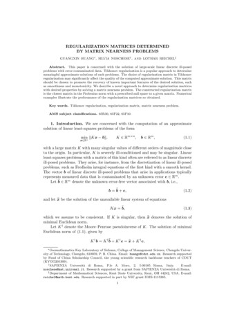
11Regularization matrices via matrix nearness 0(d)Fig. 5.1. Example 5.1: Continuous curves: Computed approximate solutions xk determined bytruncated iteration with RRGMRES using the discrepancy principle. The noise level is ν 1 · 10 4 .(a) Iterate x10 determined without regularization matrix (L I), (b) iterate x9 determined withthe regularization matrix L L1,δ P1 , (c) iterate x7 determined with the regularization matrixL L̃2 P2 , and (d) iterate x6 determined with the regularization matrix L P2 L̃2 P2 . The dashedb.curves show the desired solution xwherek(s, t) ½s(t 1),t(s 1),s t,s t.We discretize (5.2) by a Galerkin method with orthonormal box functions as test andtrial functions using the MATLAB program deriv2 from [12]. This program yields asymmetric indefinite matrix K R200 200 and a scaled discrete approximation of theb R200solution x(t) exp(t) of (5.2). Adding n1 [1, 1, . . . , 1]T yields the vector xbb . Error vectors e R200with which we compute the error-free right-hand side b : K xare constructed similarly as in Example 5.1, and the data vector b in (1.1) is obtainedfrom (1.2).Table 5.2 shows results obtained with RRGMRES for different regularizationmatrices. The performance for three noise levels is displayed. The iterations areterminated with the aid of the discrepancy principle (4.3). When L L̃2,0 , L L̃2 P2or L P2 L̃2 P2 , and the noise level is ν 1 · 10 2 , as well as when L P2 L̃2 P2 , andthe noise level is ν 1·10 3 or ν 1·10 4 , the initial residual r 0 : b Ax(0) satisfiesthe discrepancy principle and no iterations are carried out. Figure 5.2 shows computedapproximate solutions obtained for the noise level ν 1 · 10 4 with the regularizationmatrix L L̃2 P2 and without regularization matrix. Table 5.2 and Figure 5.2 showthe regularization matrix L L̃2 P2 to give the most accurate approximations of the

12G. Huang et al.reg. mat.# iterations kIL1,0L1,δ P1L̃2,0L̃2 P2P2 L̃2 P2411000IL1,0L1,δ P1L̃2,0L̃2 P2P2 L̃2 P2837110IL1,0L1,δ P1L̃2,0L̃2 P2P2 L̃2 P213226230# mat.-vec. prod.noise level v 1 · 10 2523136noise level v 1 · 10 3949246noise level v 1 · 10 414328366b k/kbkxk xxk2.4 · 10 11.1 · 10 22.6 · 10 23.1 · 10 33.1 · 10 31.1 · 10 21.5 · 10 17.3 · 10 34.6 · 10 21.9 · 10 31.7 · 10 31.1 · 10 31.0 · 10 15.6 · 10 38.0 · 10 21.4 · 10 31.2 · 10 39.5 · 10 5Table 5.2Example 5.2: Number of iterations, number of matrix-vector product evaluations with the matrixK, and relative error in approximate solutions xk determined by truncated iteration with RRGMRESusing the discrepancy principle and different regularization matrices for several noise levels.b . We remark that addition of the vector n1 to to the solution vectordesired solution xdetermined by the program deriv2 enhances the benefit of using a regularization matrixdifferent from the identity. The benefit would be even larger, if a larger multiple ofthe vector n1 were added to the solution. 2The above examples illustrate the performance of regularization matrices suggested by the theory developed in Section 2. Other combinations of nonsingularregularization matrices and orthogonal projectors also can be applied. For instance,the regularization matrix L L̃2 P1 performs as well as L L̃2 P2 when applied tothe solution of the problem of Example 5.1.6. Conclusion. This paper presents a novel method to determine regularizationmatrices via the solution of a matrix nearness problem. Numerical examples illustratethe effectiveness of the regularization matrices so obtained. While all examples usedthe discrepancy principle to determine a suitable regularized approximate solution of(1.1), other parameter choice rules also can be applied; see, e.g., [14, 20] for discussionsand references.Acknowledgment. SN is grateful to Paolo Buttà for valuable discussions andcomments on part of the present work. The authors would like to thank a referee forcomments.REFERENCES

13Regularization matrices via matrix nearness 152.12.05020406080100120140160180200(c)Fig. 5.2. Example 5.2: Continuous curves: Computed approximate solutions xk determined bytruncated iteration with RRGMRES using the discrepancy principle. The noise level is ν 1 · 10 4 .(a) Iterate x13 determined without regularization matrix (L : I), (b) iterate x3 determined withthe regularization matrix L L̃2 P2 and (c) iterate x0 determined with the regularization matrixb.L P2 L̃2 P2 . The dashed curves show the desired solution x[1] C. Brezinski, M. Redivo–Zaglia, G. Rodriguez, and S. Seatzu, Extrapolation techniques forill-conditioned linear systems, Numer. Math., 81 (1998), pp. 1–29.[2] D. Calvetti, S. Morigi, L. Reichel, and F. Sgallari, Tikhonov regularization and the L-curve forlarge discrete ill-posed problems, J. Comput. Appl. Math., 123 (2000), pp. 423–446.[3] D. Calvetti and L. Reichel, Tikhonov regularization of large linear problems, BIT, 43 (2003),pp. 263–283.[4] D. Calvetti, L. Reichel, and A. Shuibi, Invertible smoothing preconditioners for linear discreteill-posed problems, Appl. Numer. Math., 54 (2005), pp. 135–149.[5] M. Donatelli, A. Neuman, and L. Reichel, Square regularization matrices for large linear discrete ill-posed problems, Numer. Linear Algebra Appl., 19 (2012), pp. 896–913.[6] M. Donatelli and L. Reichel, Square smoothing regularization matrices with accurate boundaryconditions, J. Comput. Appl. Math., 272 (2014), pp. 334–349.[7] L. Dykes, S. Noschese, L. Reichel, Rescaling the GSVD with application to ill-posed problems,Numer. Algorithms, 68 (2015), pp. 531–545.[8] L. Eldén, A weighted pseudoinverse, generalized singular values, and constrained least squaresproblems, BIT, 22 (1982), pp. 487–501.[9] H. W. Engl, M. Hanke, and A. Neubauer, Regularization of Inverse Problems, Kluwer, Dordrecht, 1996.[10] S. Gazzola, P. Novati, and M. R. Russo, On Krylov projection methods and Tikhonov regularization, Electron. Trans. Numer. Anal., 44 (2015), pp. 83–123.[11] P. C. Hansen, Rank-Deficient and Discrete Ill-Posed Problems, SIAM, Philadelphia, 1998.[12] P. C. Hansen, Regularization tools version 4.0 for MATLAB 7.3, Numer. Algorithms, 46 (

Regularization matrices via matrix nearness problems 5 3. if B B, then hA A,Bb i 0. Proof.We have AVb 0, which shows the first property. The second property implies that AV 0, from which it follows that