Transcription
Proceedings of the 2015 Winter Simulation ConferenceL. Yilmaz, W. K. V. Chan, I. Moon, T. M. K. Roeder, C. Macal, and M. D. Rossetti, eds.APPLICATION OF METAMODELING TO THE VALUATION OF LARGE VARIABLEANNUITY PORTFOLIOSGuojun GanDepartment of MathematicsUniversity of Connecticut196 Auditorium Rd, U-3009Storrs, CT, 06269, USAABSTRACTVariable annuities are long-term investment vehicles that have grown rapidly in popularity recently. Onemajor feature of variable annuities is that they contain guarantees. The guarantees embedded in variableannuities are complex and the values of the guarantees cannot be obtained from closed-form formulas.Insurance companies rely heavily on Monte Carlo simulation to calculate the fair market values of theguarantees. Valuation and risk management of a large portfolio of variable annuities are a big challengeto insurance companies because the Monte Carlo simulation model is very time consuming. In this paper,we propose to use a metamodeling approach to speed up the valuation of large portfolios of variableannuities. Our numerical results show that the metamodeling approach can reduce the runtime significantlyand produce accurate approximations.1INTRODUCTIONA variable annuity (VA) refers to an attractive life insurance product that provides upside participation anddownside protection in both bull and bear markets. Once an investor enters into a variable annuity contractwith an insurance company, the investor agrees to make one lump-sum or a series of purchase paymentsto the insurance company and the insurance company agrees to make benefit payments to the investorbeginning immediately or at some future date. In a variable annuity contract, the investor’s money isinvested in a basket of mutual funds, which include bond funds and equity funds. When a variable annuitymatures, the benefit of the contract is equal to the market value of the accumulated purchase payments.Variable annuity has other names such as segregated fund, guaranteed investment fund, unit-linked lifeinsurance, equity-linked life insurance, or participating life insurance (Armstrong 2001)A main feature of variable annuities is that they contain guarantees. For example, almost every VAcontract contains the guaranteed minimum death benefit (GMDB) (Gerber, Shiu, and Yang 2013). VAcontracts also include the guaranteed minimum withdrawal benefit (GMWB) (Yang and Dai 2013), theguaranteed minimum maturity benefit (GMAB) (Jiang and Chang 2010), and the guaranteed minimumincome benefit (GMIB) (Bacinello, Millossovich, Olivieri, and Pitacco 2011). These guarantees are optionalin that a policyholder can purchase these guarantees for additional fees. Due to the attractive guaranteefeatures, variable annuities have grown rapidly in popularity recently. Figure 1 shows the annual sales ofvariable annuities from 2010 to 2013 in the US. From the figure we see that the annual sale of variableannuities was more than 140 billion dollars in the past few years.The guarantees embedded in variable annuities are financial guarantees that cannot be adequatelyaddressed by traditional actuarial approaches (Hardy 2000), which rely on diversification. Table 1 showsthe cash flows of a variable annuity policy with a GMWB rider under a specific economic scenario.Because of the guarantee, the policyholder can withdrawal the guaranteed amount every year even when978-1-4673-9743-8/15/ 31.00 2015 IEEE1103
201220112010Year2013Gan020406080100120140Variable Annuity Sales (in Billions)Figure 1: Variable annuity sales in the US. The numbers are in billions of dollars. (Source: LIMRA)the investment fund goes to zero. The last column shows the guarantee cash flows, which are claims paidto the policyholder by the insurance company. From the example we see that the insurance company willloss money on all policies when market goes down. Dynamic hedging (Hardy 2003) is a popular riskmanagement approach for variable annuities and is adopted by many insurance companies.Since VA contracts embedding guarantees are relatively complex, the calculation of their fair marketvalues cannot be done in closed form except for special cases (Gerber and Shiu 2003, Feng and Volkmer2012). In practice, insurance companies rely on the Monte Carlo simulation method to determine the fairmarket values of VA contracts. However, using the Monte Carlo simulation method to value a large portfolioof VA contract is time consuming because every VA contract needs to be projected over many scenariosfor a long time horizon. For example, using a Monte Carlo simulation method with 1,000 scenarios and360 monthly time steps to calculate the fair market value of a portfolio consisting of 100,000 VA policiesinvolves the following number of cash flow projections:100, 000 1, 000 360 3.6 1010 .If a computer can process 200,000 projections per second, then it would take this computer 50 hours tofinish the calculation. That is only the runtime for calculating the fair market value under a single marketcondition. To calculate the fair market values under 100 different market conditions, it would take thiscomputer 5,000 hours to complete the calculation.To make dynamic hedging work for a large portfolio of VA policies, an insurance company needs tocalculate the Greeks (e.g., dollar Delta and dollar Rho) of the big portfolio on a daily basis in order toincorporate the changes in the portfolio and the market. In particular, the insurance company needs tocomplete the calculation of the Greeks over night between today’s market close and tomorrow’s marketopen. In order to complete the computationally intensive calculation, insurance companies employ manycomputers to do the calculation. For example, GPUs (Graphics Processing Unit) have been used to valueVA contracts (Phillips 2012, NVIDIA 2012).Although using many computers or GPUs can speed up the calculation, this approach is not scalable.In other words, if the number of VA policies in a portfolio doubles, then the insurance company needsto double the number of computers or GPUs in order to complete the calculation within the same timeinterval. In addition, buying or renting many computers or GPUs is expensive and can cost the insurancecompany a lot of money annually.1104
GanTable 1: Cash flows of a variable annuity policy with a GMWB rider under a specific economic scenario.In this sample variable annuity policy, the initial investment is 100,000 dollars, the GMWB amount is equalto the initial investment, and the policyholder is allowed to withdrawal 8% of the initial investment untilthe initial investment is ,4090000000RemainingBenefitGuaranteeCash 008,0008,0008,0004,000In this paper, we apply a metamodeling approach to address the computational problem mentionedabove. In particular, we adopt a metamodel by using a Latin hypercube sampling method (McKay, Beckman,and Conover 1979, Pistone and Vicario 2010, Petelet, Iooss, Asserin, and Loredo 2010, Viana 2013) andthe ordinary kriging model (Isaaks and Srivastava 1990).The remaining of the paper is structured as follows. Section 2 gives a brief review of simulationmetamodeling and its application in finance. Section 3 introduces a Latin hypercube sampling methodused to select representative VA contracts and the ordinary kriging model. Section 3 also presents somenumerical results of the proposed metamodel. Section 4 concludes the paper and gives a survey of futurework.2METAMODELINGIn simulation modeling, a metamodel refers to a model of a simulation model (Friedman 1996). Onemain reason for building a model of a simulation model is that the simulation model is complicate andcomputationally intensive. Metamodels of a simulation model are much simpler and more computationallyefficient than the simulation model. Metamodels are sometimes called response surface models or surrogatemodels.Building a metamodel of a simulation model involves three steps: first, we use an experimental designmethod to select a small set of sample points from the input domain; second, we run the simulationmodel to generate outputs at these selected sample points; third, we choose an appropriate metamodelform and estimate the parameters of the metamodel using the selected sample points and the outputs ofthe simulation model at the selected sample points. The experimental design method and the metamodelare two interrelated components of metamodeling.During the past six decades, many papers on metamodelling and its applications have been published.Early works in this area include (Kleijnen 1975), (Franke 1982), (Hoerl 1985), (Barton 1992), (Laslett1994), (Barton 1994), (Madu and Kuei 1994), (Barton 1998), to name just a few. Kleijnen (1975) introduced1105
Ganthe concept of metamodels for simulation models. Barton (1994) presented a review of metamodels forstudying the behavior of computer simulations during that time. In particular, Barton reviewed severalmodeling approaches such as spline models, radial basis functions, kernel methods, and spatial correlationmodels. Barton (1998) discussed other metamodel types such as neural network metamodels.Recent works in this area include (Kleijnen and Deflandre 2006), (Wu, Chen, Hu, Zhang, and Liang2008), (Kleijnen 2009), (Ankenman, Nelson, and Staum 2010), (Khuri and Mukhopadhyay 2010), (Yin, Ng,and Ng 2011), (Razavi, Tolson, and Burn 2012), (Wei, Wu, and Chen 2012), and (Zhao, Yue, Liu, Gao, andZhang 2014), to name just a few. Kleijnen (2009) presented a review of the Kriging metamodel. Ankenman,Nelson, and Staum (2010) extended the basic theory of Kriging to the stochastic simulation setting. Khuriand Mukhopadhyay (2010) provided a survey of the development of response surface methodology since itsintroduction in the early 1950s. Razavi, Tolson, and Burn (2012) presented a wide variety of metamodelingmethods with an emphasis on the water resources field.A number of books have been devoted to metamodels, response surface methodologies, and surrogatemodels: (Box and Draper 1987), (Khuri and Cornell 1987), (Friedman 1996), (Shore 2005), (Khuri 2006),(Box and Draper 2007), (Forrester, Sobester, and Keane 2008), (Myers, Montgomery, and Anderson-Cook2009), and (Das 2014). Friedman (1996) presented a diverse set of scholarly materials relevant to thestudy of simulation metamodels, including usage, applications, and methodology of metamodels. Box andDraper (2007) is a successor volume to Box and Draper (1987) and covers many topics on response surfacemodels. Das (2014) is an introductory book devoted to robust response surface methodology and containsa review of the existing literature on response surface methodology.The concept of metamodeling has been applied to financial engineering recently. In (Baysal, Nelson,and Staum 2008), the authors used Latin hypercube designs and kriging to simulate hedging and tradingstrategies under nested simulation. Liu and Staum (2009) and Liu and Staum (2010) used stochastic krigingto estimate expected shortfall of a portfolio. Gan (2013) used a data clustering method (Gan 2011) and theordinary kriging method to estimate the fair market values of a portfolio of variable annuities. Salle andYildizoglu (2014) applied the kriging model to approximate two well known economic models. Gan andLin (2015) used a data clustering method and a universal kriging method developed for functional data toestimate the fair market values of a portfolio of variable annuities under nested simulation.3AN APPLICATION OF METAMODELING TO VARIABLE ANNUITYIn this section, we apply a metamodeling method to attack the computational problem arising from thevariable annuity area. In this example, we use Latin hypercube sampling and kriging. The kriging methodis a popular metamodeling method and the Latin hypercube sampling method works well with the krigingmethod (Baysal, Nelson, and Staum 2008).3.1 Latin Hypercube SamplingLatin hypercube sampling (LHS) is a statistical method for generating plausible design points from multipledimensional spaces that are used to conduct computer experiments. Figure 2 gives two examples of Latinhypercube designs with 4 points on a 2-dimensional area. From the figure we see that there is only onesample point in each row and each column. For more information about LHS, readers are referred to(McKay, Beckman, and Conover 1979), (Liefvendahl and Stocki 2006), (Minasny and McBratney 2006),(Pistone and Vicario 2010), (Petelet, Iooss, Asserin, and Loredo 2010), and (Viana 2013).When the number of divisions and the number of variables increase, the number of Latin hypercubesincreases exponentially (McKay and Wanless 2008). For example, there are64 4! (3!)3 331, 776Latin hypercubes with 4 divisions and 3 variables. As a result, one way to find a good Latin hypercubedesign is to generate Latin hypercube samples randomly and select the best one from the samples.1106
Gan(a)(b)Figure 2: Two examples of Latin hypercube designs with 4 divisions and 2 variables.Now let us introduce a LHS method for selecting representative VA policies, which are describedby both categorical and numerical variables. The LHS method introduced here is able to handle bothnumerical and categorical variables. There are several ways to select an optimal Latin hypercube design(Liefvendahl and Stocki 2006). Here we select an optimal Latin hypercube design by maximizing theminimum distances.To describe the LHS method, we assume that a VA contract is characterized by d attributes (e.g.,gender, age, account value, etc.) and that the first d1 attributes are numerical and the remaining d2 d d1attributes are categorical. For j 1, 2, . . . , d1 , let L j and H j denote the minimum and maximum values thatthe jth numerical variable can take. That is,L j min{x j : x X},H j max{x j : x X},(1)where x j denotes the jth component of x and X {x1 , x2 , · · · , xn } denote the portfolio of VA contracts.For j d1 1, d1 2, . . ., d, let N j denote the number of distinct values that the jth categorical variablecan take, i.e.,(2)N j {x j : x X} ,where · denote the number of elements in a set.Suppose that we want to generate a Latin hypercube design with k design points, where k 2. To dothat, we first divide the range of each of the d1 numerical variable into k divisions. For each l 1, 2, . . . , k,the lth division of the jth dimension is given by 3 Hj L j1 Hj L j,Lj l Il L j l .2k 12k 1Sincek[ Hj LjHj Lj, Hj [L j , H j ],Il L j 2(k 1)2(k 1)l 1the union of the k divisions covers the whole range of the jth variable. For each of the remaining categoricalvariables, we just treat each category as a division.Let H be a set of d-dimensional points defined to beH {(a1 , a2 , . . . , ad )}such that for j 1, 2, . . . , d1 , Hj L ja j L j (l 1), l 1, 2, . . . , k ,k 11107(3)
Ganand for j d1 1, d1 2, . . . , d, a j A jl , l 1, 2, . . . , N j ,where A j1 , A j2 , . . ., A jN j are the distinct categories of the jth variable and L j , H j , and N j are defined inEquations (1) and (2). There are many points in the set H . In fact, we have H kd1d N j.j d1 1The first step of the LHS method is to select k points from the set H with the best score, which is tobe defined. Let H be a subset of H with k elements. The score of the set H is defined to be the minimumdistance between any pairs of distinct points in H. That is,S(H) min {M(a, b) : a H, b H, a 6 b} ,(4)where M(a, b) is the distance between a and b given byd1M(a, b) d(k 1) a j b j Hj Lj δ (a j , b j ),j 1j d1 1(5)where a j and b j are the jth components of a and b, respectively, and δ (·, ·) is defined in Equation (10).The larger the score, the better the Latin hypercube design. An optimal Latin hypercube design with kpoints is defined as(6)H argmax S(H).H H , H kSince the set H contains huge number of points, finding an optimal Latin hypercube design with kpoints from H is not easy. To find such an optimal Latin hypercube design, we randomly generate many(e.g., 500) Latin hypercube designs and select the one with the largest score. To generate a random Latinhypercube design H {a1 , a2 , . . . , ak } with k points, we proceed as follows:1. For each j 1, 2, . . . , d1 , we randomly generate k uniform real numbers from the interval [0, 1].Suppose that these random numbers are r j1 , r j2 , . . ., r jk . Since these numbers are random realnumbers, they are mutually distinct in general. We sort the k real numbers in an ascending ordersuch thatr ji1 r jr2 · · · r jrk ,where (i1 , i2 , . . . , ik ) is a permutation of (1, 2, . . . , k). Then we define the first d1 coordinates of thek design points asa jl L j (il 1)Hj L j,k 1j 1, . . . , d1 , l 1, . . . , k.For each j 1, 2, . . . , d1 , the coordinates of the k design points at the jth dimension are mutuallydistinct.2. For each j d1 1, d1 2, . . . , d, we randomly generate k uniform integers from {1, 2, . . . , N j }. Forportfolios of variable annuity policies, we usually have k N j , that is, the number of design pointsis larger than the number of values that a categorical variable can take. Suppose that these randomintegers are i1 , i2 , . . . , ik . Then we define the remaining d2 coordinates of the k design points asa jl A jil ,j d1 1, . . . , d, l 1, . . . , k,where A j1 , A j2 , . . ., A jN j are the distinct categories of the jth variable.1108
GanOnce we find a Latin hypercube design H {a 1 , a 2 , . . . , a k } using the above procedure. The secondstep of the LHS method is to find k representative VA policies that are close to the k design points in H .In particular, the VA policy that is close to a i is determined byzi argmin M(a i , x),i 1, 2, . . . , k,x Xwhere M(·, ·) is defined in Equation (5).3.2 Ordinary KrigingWe use the ordinary kriging method (Isaaks and Srivastava 1990) to estimate the fair market value andthe Greeks (e.g., sensitivities of the fair market values) of the whole portfolio from the representative VApolicies.Let z1 , z2 , . . ., zk be the representative VA contracts obtained from the clustering algorithm. For everyj 1, 2, . . . , k, let y j be the fair value of z j that is calculated by the Monte Carlo method. Then we use theKriging method to estimate the fair value of the VA contract xi askŷi wi j · y j ,(7)j 1where wi1 , wi2 , . . . , wik are the Kriging weights.The Kriging weights wi1 , wi2 , . . . , wik are obtained by solving the V11 · · · V1k 1wi1 . . . . . . · . Vk1 · · · Vkk 1 wik 1 ··· 1 0θifollowing linear equation system Di1. . (8) ,Dik 1where θi is a control variable used to make sure the sum of the Kriging weights is equal to one, 3Vrs α exp D(zr , zs ) , r, s 1, 2, . . . , k,βand 3Di j α exp D(xi , z j ) ,βj 1, 2, . . . , k.Here α 0 and β 0 are two parameters, and the distance function D(·, ·) is defined asvuddu 1D(x, y) t (xh yh )2 δ (xh , yh ),(9)h d1 1h 1where xh and yh are the hth component of x and y, respectively, and δ (·, ·) is the simple matching distancedefined as 0, if xh yh ,δ (xh , yh ) (10)1, if xh 6 yh .Since D(zr , zs ) 0 for all 1 r s k, the above linear equation system has a unique solution (Isaaksand Srivastava 1990).1109
GanThe fair value of the portfolio X is equal to the sum of the fair values of all VA contracts in X, i.e.,nnkkŶ ŷi wi j · y j i 1 j 1i 1where w j · y j,(11)j 1nw j wi j .i 1The fair value Ŷ of the portfolio can be calculatedfollowing linear equation system V11 · · · V1k 1 . . . . . · Vk1 · · · Vkk 1 1 ··· 1 0whereefficiently by solving w1 , w2 , . . ., wk from the w1. . wk θ D1. . ,Dk n(12)nD j Di j ,j 1, 2, . . . , k.i 1In fact, Equation (12) is obtained by summing both sides of Equation (8) from i 1 to n.3.3 Numerical ResultsIn this subsection, we present some numerical results of using the metamodel for VA portfolio valuation.To do the test, we follow the setup used in (Gan 2013). We generate a portfolio of 200,000 synthetic VAcontracts. The attributes and their ranges of values are shown in Table 2. For each synthetic VA contract,the value of an attribute is generated from a uniform distribution with the corresponding range given inTable 2.Table 2: Variable annuity attributes and their ranges of values. Here GMDB and GMWB refer to guaranteedminimum death benefit and guaranteed minimum withdrawal benefit, which are two major features of variableannuities.AttributeValuesGuarantee typeGenderAgeAccount valueGMWB withdrawal rateMaturity{GMDB only, GMDB GMWB}{Male, Female}{20, 21, 22, . . ., 60}[10000, 500000]{0.04, 0.05, 0.06, 0.07, 0.08}{10, 11, 12, . . ., 25}We use the metamodel to estimate the fair market value, dollar Delta, and dollar Rho of the wholeportfolio. In all the test cases, we used 500 iterations in the LHS method. In other words, 500 Latinhypercube designs are randomly generated and the one with the largest score is selected.In our test, we used the LHS method to select a set of representative VA policies. Then we usedthe ordinary kriging method to estimate the fair market value, dollar Delta, and dollar Rho of the wholeportfolio. In the ordinary kriging method, we set α 0 and β to be the 95th percentile of all distancesbetween pairs of the representative VA policies as suggested in (Isaaks and Srivastava 1990). The accuracyof the metamodel is summarized in Table 3. The first row (MC) shows the fair market value, dollar Delta,1110
Ganand dollar Rho of the portfolio calculated by the Monte Carlo simulation model. The second row and thethird row shows the numbers estimated by the metamodel. The last four rows show the dollar differenceand the percentage difference. From the tables we see than most of the percentage differences are less than0.5%.Table 3: The fair market values, dollar Deltas, and dollar Rhos calculated by the Monte Carlo simulationmodel and those estimated by the metamodel with different number of representative VA policies. Numbersin the first five rows are in dollars. Numbers in brackets are negative numbers.Fair Market ValueDollar DeltaDollar C)/MC(LHS500-MC)/MCTable 4: Runtime used by the Monte Carlo simulation model and the metamodel with different number ofrepresentative VA policies. The numbers are in seconds. The LHS, MC, Kriging rows denote the runtimeused by the Latin hypercube sampling method, the Monte Carlo simulation model, and the ordinary krigingmethod, respectively.Number of Rep. PoliciesEntire 75.3826.8NA1942.22NATotal12.5152.651942.22Table 4 shows the runtime used by the Monte Carlo simulation model and that used by the metamodel.From the table we see that the metamodel is much faster than the Monte Carlo simulation model for valuingthe portfolio. It took the Monte Carlo simulation model more than 30 minutes to calculate the fair marketvalue, dollar Delta, and dollar Rho of the portfolio. In contrast, it took the metamodel less than one minuteto produce accurate estimates of these numbers.Although the VA policies considered in the numerical experiments are much simpler than the real VApolicies, the numerical results show that metamodeling is a promising approach to address the computationalproblem arising from the VA area.4CONCLUSIONSFor an insurance company that has a big VA portfolio, a major challenge in risk management of the VAbusiness is to calculate the fair market value and the Greeks of the VA portfolio in an efficient way. In thispaper, we proposed a metamodeling approach to address the computational problem from the perspectiveof mathematical modeling instead of hardware. The idea of the metamodeling approach is to first select asmall set of representative policies, then price the representative policies, and finally estimate the value of1111
Ganthe whole portfolio. The method is efficient in that only a small set of representative policies is requiredto be priced by the time-consuming Monte Carlo simulation model.To test the usefulness of the metamodeling method, we created a synthetic portfolio of VA policiesand compared the accuracy and speed of the metamodel and the Monte Carlo simulation model usingthe synthetic portfolio. Our numerical results indicate that the metamodeling method is computationallyefficient and is able to produce accurate approximations.The metamodeling approach can be useful for insurance companies that have a VA business. Oursimple numerical experiments show that the metamodeling approach has the potential to reduce the runtimesignificantly. In practice, the simulation model used by insurance companies is much more complex thanthe one used in this paper. For example, monthly time steps are usually used in practice and the cashflow projection is often complex for real variable annuity policies. The metamodeling approach can reducethe runtime even more in real applications than in the toy example presented in the paper. In addition,the metamodeling approach can also be used to address other computationally intensive issues such ascalculating the economic capitals of a portfolio of variable annuities.In future, we would like to test other experimental design methods and metamodeling techniques. Inparticular, we would like to conduct a comprehensive comparison of various experimental design methods,such as factorial design (Alam, McNaught, and Ringrose 2004), and metamodeling techniques, such asresponse surface methodology (Myers, Montgomery, and Anderson-Cook 2009).REFERENCESAlam, F. M., K. R. McNaught, and T. J. Ringrose. 2004. “A comparison of experimental designs in thedevelopment of a neural network simulation metamodel”. Simulation Modelling Practice and Theory 12(78): 559 – 578. Simulation in Operational Research.Ankenman, B., B. L. Nelson, and J. Staum. 2010. “Stochastic Kriging for Simulation Metamodeling”.Operations Research 58 (2): 371–382.Armstrong, M. 2001. “The reset decision for segregated fund maturity guarantees”. Insurance: Mathematicsand Economics 29:257–269.Bacinello, A., P. Millossovich, A. Olivieri, and E. Pitacco. 2011. “Variable annuities: A unifying valuationapproach”. Insurance: Mathematics and Economics 49 (3): 285–297.Barton, R. 1994, Dec. “Metamodeling: a state of the art review”. In Winter Simulation ConferenceProceedings, 237–244.Barton, R. R. 1992. “Metamodels for Simulation Input-output Relations”. In Proceedings of the 24thConference on Winter Simulation, WSC ’92, 289–299: ACM.Barton, R. R. 1998. “Simulation Metamodels”. In Proceedings of the 30th Conference on Winter Simulation,WSC ’98, 167–176. Los Alamitos, CA, USA: IEEE Computer Society Press.Baysal, R., B. Nelson, and J. Staum. 2008, Dec. “Response surface methodology for simulating hedgingand trading strategies”. In Simulation Conference, 2008. WSC 2008. Winter, 629–637.Box, G. E. P., and N. R. Draper. 1987. Empirical Model-Building and Response Surfaces. Hoboken, NJ:Wiley.Box, G. E. P., and N. R. Draper. 2007. Response Surfaces, Mixtures, and Ridge Analyses. 2nd ed. Hoboken,NJ: Wiley.Das, R. N. 2014. Robust Response Surfaces, Regression, and Positive Data Analyses. Boca Raton, FL:CRC Press.Feng, R., and H. Volkmer. 2012. “Analytical calculation of risk measures for variable annuity guaranteedbenefits”. Insurance: Mathematics and Economics 51 (3): 636–648.Forrester, A., A. Sobester, and A. Keane. 2008. Engineering Design via Surrogate Modelling: A PracticalGuide. West Sussex, UK: Wiley.Franke, R. 1982. “Scattered Data Interpolation: Tests of Some Method”. Mathematics of Computation 38(157): 181–200.1112
GanFriedman, L. W. 1996. The Simulation Metamodel. Norwell, MA, USA: Kluwer Academic Publishers.Gan, G. 2011. Data Clustering in C : An Object-Oriented Approach. Data Mining and KnowledgeDiscovery Series. Boca Raton, FL, USA: Chapman & Hall/CRC Press.Gan, G. 2013. “Application of data clustering and machine learning in variable annuity valuation”. Insurance:Mathematics and Economics 53 (3): 795–801.Gan, G., and X. S. Lin. 2015. “Valuation of large variable annuity portfolios under nested simulation: Afunctional data approach”. Insurance: Mathematics and Economics 62:138–150.Gerber, H., and E. Shiu. 2003. “Pricing Lookback Options and Dynamic Guarantees”. North AmericanActuarial Journal 7 (1): 48–67.Gerber, H., E. Shiu, and H. Yang. 2013. “Valuing equity-linked death benefits in jump diffusion models”.Insurance: Mathematics and Economics 53 (3): 615–623.Hardy, M. 2000. “Hedging and reserving for single premium segregated fund contracts”. North AmericanActuarial Journal 4 (2): 63–74.Hardy, M. 2003. Investment Guarantees: Modeling and Risk Management for Equity-Linked Life Insurance.Hoboken, New Jersey: John Wiley & Sons, Inc.Hoerl, R. W. 1985. “Ridge Analysis 25 Years Later”. The American Statistician 39 (3): 186–192.Isaaks, E., and R. Srivastava. 1990. An Introduction to Applied Geostatistics. Oxford, UK: Oxford UniversityPress.Jiang, S., and M. Chang. 2010. “Variable Annuity with Guarantees: Valuation and Simulation”. Journal ofMoney, Investment and Banking 14:74–83.Khuri, A. I. (Ed.) 2006. Response Surface Methodology And Related Topics. Singapore: World Scientific.Khuri, A. I., and J. A. Cornell. 1987. Response Surfaces: Designs
Storrs, CT, 06269, USA ABSTRACT Variable annuities are long-term investment vehicles that have grown rapidly in popularity recently. One major feature of variable annuities is that they contain guarantees. The guarantees embedded in variable . Variable annuity has other names such as segregated fund, guaranteed investment fund, unit-linked .