Transcription
Introduction toComsol MultiphysicsVERSION 4.4
IntroductionToCOMSOLMultiphysics.book Page i Tuesday, January 14, 2014 4:03 PMIntroduction to COMSOL Multiphysics 1998–2013 COMSOLProtected by U.S. Patents 7,519,518; 7,596,474; 7,623,991; and 8,457,932. Patents pending.This Documentation and the Programs described herein are furnished under the COMSOL Software LicenseAgreement (www.comsol.com/comsol-license-agreement) and may be used or copied only under the terms of thelicense agreement.COMSOL, COMSOL Multiphysics, Capture the Concept, COMSOL Desktop, and LiveLink are either registeredtrademarks or trademarks of COMSOL AB. All other trademarks are the property of their respective owners, andCOMSOL AB and its subsidiaries and products are not affiliated with, endorsed by, sponsored by, or supported bythose trademark owners. For a list of such trademark owners, see www.comsol.com/trademarks.Version:December 2013COMSOL 4.4Contact InformationVisit the Contact COMSOL page at www.comsol.com/contact to submit general inquiries, contactTechnical Support, or search for an address and phone number. You can also visit the WorldwideSales Offices page at www.comsol.com/contact/offices for address and contact information.If you need to contact Support, an online request form is located at the COMSOL Access page atwww.comsol.com/support/case.Other useful links include: Support Center: www.comsol.com/support Product Download: www.comsol.com/product-download Product Updates: www.comsol.com/support/updates COMSOL Community: www.comsol.com/community Events: www.comsol.com/events COMSOL Video Gallery: www.comsol.com/video Support Knowledge Base: www.comsol.com/support/knowledgebasePart number: CM010004
IntroductionToCOMSOLMultiphysics.book Page i Tuesday, January 14, 2014 4:03 PMContentsIntroduction . . . . . . . . . . . . . . . . . . . . . . . . . . . . . . . . . . . . . . . . . . . . 1COMSOL Desktop . . . . . . . . . . . . . . . . . . . . . . . . . . . . . . . . . . . . 2Example 1: Structural Analysis of a Wrench . . . . . . . . . . . . . . . . 24Example 2: The Busbar—A Multiphysics Model . . . . . . . . . . . . . 46Advanced Topics . . . . . . . . . . . . . . . . . . . . . . . . . . . . . . . . . . . . . . 74Parameters, Functions, Variables and Couplings. . . . . . . . . . 74Material Properties and Material Libraries. . . . . . . . . . . . . . . 78Adding Meshes . . . . . . . . . . . . . . . . . . . . . . . . . . . . . . . . . . . . . 80Adding Physics . . . . . . . . . . . . . . . . . . . . . . . . . . . . . . . . . . . . . 82Parametric Sweeps. . . . . . . . . . . . . . . . . . . . . . . . . . . . . . . . . 103Parallel Computing . . . . . . . . . . . . . . . . . . . . . . . . . . . . . . . . . 111Appendix A—Building a Geometry . . . . . . . . . . . . . . . . . . . . . . 114Appendix B—Keyboard and Mouse Shortcuts . . . . . . . . . . . . . 128Appendix C—Language Elements and Reserved Names . . . . 131Appendix D—File Formats . . . . . . . . . . . . . . . . . . . . . . . . . . . . . 143Appendix E—Connecting with LiveLink Add-Ons. . . . . . . . 149Contents i
IntroductionToCOMSOLMultiphysics.book Page ii Tuesday, January 14, 2014 4:03 PMii Contents
IntroductionToCOMSOLMultiphysics.book Page 1 Tuesday, January 14, 2014 4:03 PMIntroductionRead this book if you are new to COMSOL Multiphysics . It provides a quickoverview of the COMSOL environment with examples that show you how to usethe COMSOL Desktop user interface.If you have not yet installed the software, install it now according to theinstructions at: www.comsol.com/product-download.In addition to this book, an extensive documentation set is available afterinstallation. A video gallery with tutorials can be found at:www.comsol.com/video.Introduction 1
IntroductionToCOMSOLMultiphysics.book Page 2 Tuesday, January 14, 2014 4:03 PMCOMSOL Desktop QUICK ACCESS TOOLBAR—Use thesebuttons for access to functionality such as fileopen/save, undo/redo, copy/paste, and delete.RIBBON—The ribbon tabs have buttonsand drop-down lists for controlling allsteps of the modeling process.MODEL BUILDERTOOLBARMODEL TREE—The modeltree gives an overview of themodel and all the functionalityand operations needed forbuilding and solving a modelas well as processing theresults.2 COMSOL Desktop MODEL BUILDERWINDOW—The Model Builderwindow with its model tree andthe associated toolbar buttonsgives you an overview of themodel. The modeling processcan be controlled fromcontext-sensitive menusaccessed by right-clicking a node.SETTINGS WINDOW—Clickany node in the model tree tosee its associated settingswindow displayed next to theModel Builder.
IntroductionToCOMSOLMultiphysics.book Page 3 Tuesday, January 14, 2014 4:03 PMGRAPHICS WINDOW TOOLBARGRAPHICS WINDOW—The Graphics window presentsinteractive graphics for the Geometry, Mesh, and Results.Operations include rotating, panning, zooming, andselecting. It is the default window for most Results andvisualizations.INFORMATION WINDOWS—The Information windows will display vitalmodel information during the simulation, such as the solution time, solutionprogress, mesh statistics, solver logs, and, when available, Results Tables.COMSOL Desktop 3
IntroductionToCOMSOLMultiphysics.book Page 4 Tuesday, January 14, 2014 4:03 PMThe screen shot on the previous pages is what you will see when you first startmodeling in COMSOL. COMSOL Desktop provides a complete and integratedenvironment for physics modeling and simulation. You can customize it to yourown needs. The desktop windows can be resized, moved, docked, and detached.Any changes you make to the layout will be saved when you close the session andused again the next time you open COMSOL. As you build your model,additional windows and widgets will be added. (See page 20 for an example of amore developed desktop). Among the available windows and user interfacecomponents are the following:Quick Access ToolbarThe Quick Access Toolbar gives access to functionality such as Open, Save, Undo,Redo, Copy, Paste, and Delete. You can customize its content from theCustomize Quick Access Toolbar list.RibbonThe ribbon at the top of the desktop gives access to commands used to completemost modeling tasks. The ribbon is only available in the Windows version of theCOMSOL Desktop environment and is replaced by menus and toolbars in theOS X and Linux versions.Settings WindowThis is the main window for entering all of the specifications of the modelincluding the dimensions of the geometry, properties of the materials, boundaryconditions and initial conditions, and any other information that the solver will4 COMSOL Desktop
IntroductionToCOMSOLMultiphysics.book Page 5 Tuesday, January 14, 2014 4:03 PMneed to carry out the simulation. The picture below shows the settings window forthe Geometry node.Plot WindowsThese are the windows for graphical output. In addition to the Graphics window,Plot windows are used for Results visualization. Several Plot windows can be usedto show multiple results simultaneously. A special case is the Convergence Plotwindow, an automatically generated Plot window that displays a graphicalindication of the convergence of the solution process while a model is running.Information WindowsThese are the windows for non-graphical information. They include: Messages: Various information about events of the current COMSOLsession is displayed in this window. Progress: Progress information from the solver in addition to stop buttons. Log: Information from the solver such as number of degrees of freedom,solution time and solver iteration data.COMSOL Desktop 5
IntroductionToCOMSOLMultiphysics.book Page 6 Tuesday, January 14, 2014 4:03 PM Table: Numerical data in table format as defined in the Results branch. External Process: Provides a control panel for cluster, cloud and batch jobs.Other Windows Add Material and the Material Browser: Access the material propertylibraries. The Material Browser enables editing of material properties. Selection List: A list of geometry objects, domains, boundaries, edges andpoints that are currently available for selection.The More Windows drop-down list in the Home tab of the ribbon gives youaccess to all COMSOL Desktop windows. (On OS X and Linux , you will findthis in the Windows menu.)Progress Bar with Cancel ButtonThe Progress Bar with a button for canceling the current computation, if any, islocated in the lower right-hand corner of the COMSOL Desktop interface.Dynamic HelpThe Help window provides context dependent help texts about windows andmodel tree nodes. If you have the Help window open in your desktop (by typingF1 for example) you will get dynamic help (in English only) when you click a nodeor a window. From the Help window you can search for other topics such as menuitems.6 COMSOL Desktop
IntroductionToCOMSOLMultiphysics.book Page 7 Tuesday, January 14, 2014 4:03 PMPrefe re n c esPreferences are settings that affect the modeling environment. Most are persistentbetween modeling sessions, but some are saved with the model. You accessPreferences from the File menu.In the Preferences window you can change settings such as graphics rendering,number of displayed digits for Results, maximum number of CPU cores used forcomputations, or paths to user-defined model libraries. Take a moment to browseyour current settings to familiarize yourself with the different options.There are three graphics rendering options available: OpenGL , DirectX , andSoftware Rendering. DirectX is not available in OS X or Linux but is availablein Windows if you choose to install the DirectX runtime libraries duringinstallation. If your computer doesn’t have a dedicated graphics card, you mayhave to switch to Software Rendering for slower but fully functional graphics. Alist of recommended graphics cards can be found at:www.comsol.com/system-requirementsCOMSOL Desktop 7
IntroductionToCOMSOLMultiphysics.book Page 8 Tuesday, January 14, 2014 4:03 PMCre a t ing a New M ode lYou can create a new model guided by the Model Wizard or start from a BlankModel.C REATINGAM ODEL G UIDEDBY THEM ODEL W IZARDThe Model Wizard will guide you in setting up the space dimension, physics, andstudy type, in a few steps:1 Start by selecting the space dimension for your model component: 3D, 2DAxisymmetric, 2D, 1D Axisymmetric, or 0D.2 Now, add one or more physics interfaces. These are organized in a number ofPhysics branches in order to make them easy to locate. These branches do notdirectly correspond to products. When products are added to your COMSOL8 COMSOL Desktop
IntroductionToCOMSOLMultiphysics.book Page 9 Tuesday, January 14, 2014 4:03 PMinstallation, one or more branches will be populated with additional physicsinterfaces.3 Select the Study type that represents the solver or set of solvers that will be usedfor the computation.Finally, click Done. The desktop is now displayed with the model treeCOMSOL Desktop 9
IntroductionToCOMSOLMultiphysics.book Page 10 Tuesday, January 14, 2014 4:03 PMconfigured according to the choices you made in the Model Wizard.C REATINGAB LANK M ODELThe Blank Model option will open the COMSOL Desktop interface without anyComponent or Study. You can right-click the model tree to add a Component ofa certain space dimension, a physics interface, or a Study.The Ribb on and Quick Access ToolbarThe ribbon tabs on the COMSOL Desktop environment reflect the modelingworkflow and gives an overview of the functionality available for each modelingstep.The Home tab has buttons for the most common operations for making changesto a model and for running simulations. Examples include changing modelparameters for a parameterized geometry, reviewing material properties andphysics, building the mesh, running a study, and visualizing the simulation results.There are standard tabs for each of the main steps in the modeling process. Theseare ordered from left to right according to the workflow: Definitions, Geometry,Physics, Mesh, Study, and Results.Contextual tabs are shown only if and when they are needed, such as the 3D PlotGroup tab which is shown when the corresponding plot group is added or whenthe node is selected in the model tree.Modal tabs are used for very specific operations, when other operations in theribbon may become temporarily irrelevant. An example is the Work Plane modaltab. When working with Work Planes, other tabs are not shown since they do notpresent operations relevant to.10 COMSOL Desktop
IntroductionToCOMSOLMultiphysics.book Page 11 Tuesday, January 14, 2014 4:03 PMT HE R IBBONVS .T HE M ODEL B UILDERThe ribbon gives quick access to available commands and complements the modeltree in the Model Builder window. Most of the functionally accessed from theribbon is also accessible from contextual menus by right-clicking nodes in themodel tree. Certain operations are only available from the ribbon, such as selectingwhich desktop window to display. In the COMSOL Desktop interface for OS Xand Linux , this functionality is available from toolbars which replace the ribbonon these platforms. There are also operations that are only available from themodel tree, such as reordering and disabling nodes.T HE Q UICK A CCESS TOOLBARThe Quick Access Toolbar contains a set of commands that are independent of theribbon tab that is currently displayed. You can customize the Quick AccessToolbar: you can add most commands available in the File menu, commands forundoing and redoing recent actions, for copying, pasting, duplicating, anddeleting nodes in the model tree. You can also choose to position the QuickAccess Toolbar above or below the ribbon.OS XANDL INUX In the COMSOL Desktop environment for OS X and Linux , the ribbon isreplaced by a set of menus and toolbars:T h e M o d e l B u i l d e r a n d t h e M o d e l Tre eThe Model Builder is the tool where you define the model and its components:how to solve it, the analysis of results, and the reports. You do that by building amodel tree.You build a model by starting with the default model tree, adding nodes, andediting the node settings.All of the nodes in the default model tree are top-level parent nodes. You canright-click on them to see a list of child nodes, or subnodes, that you can addbeneath them. This is the means by which nodes are added to the tree.When you click on a child node, then you will see its node settings in the settingswindow. It is here that you can edit node settings.COMSOL Desktop 11
IntroductionToCOMSOLMultiphysics.book Page 12 Tuesday, January 14, 2014 4:03 PMIt is worth noting that if you have the Help window open (which is achieved eitherby selecting Help from the File menu, or by pressing the function key F1), thenyou will also get dynamic help (in English only) when you click on a node.T HE R OOT , G LOBAL D EFINITIONS ,ANDR ESULTS N ODESA model tree always has a root node (initiallylabeled Untitled.mph), a Global Definitionsnode, and a Results node. The label on theroot node is the name of the multiphysicsmodel file, or MPH file, that this model issaved to. The root node has settings for authorname, default unit system, and more.The Global Definitions node is where you define parameters, variables, functions,and couplings that can be used throughout the model tree. They can be used, forexample, to define the values and functional dependencies of material properties,forces, geometry, and other relevant features. The Global Definitions node itselfhas no settings, but its child nodes have plenty of them.The Results node is where you access the solution after performing a simulationand where you find tools for processing the data. The Results node initially hasfive subnodes: Data Sets: contains a list of solutions youcan work with. Derived Values: defines values to be derivedfrom the solution using a number ofpostprocessing tools. Tables: a convenient destination for theDerived Values or for Results generated byprobes that monitor the solution inreal-time while the simulation is running. Export: defines numerical data, images, and animations to be exported tofiles. Reports: contains automatically generated or custom reports about themodel in HTML or Microsoft Word format.To these five default subnodes, you may also add additional Plot Group subnodesthat define graphs to be displayed in the Graphics window or in Plot windows.Some of these may be created automatically, depending on the type of simulationsyou are performing, but you may add additional figures by right-clicking on theResults node and choosing from the list of plot types.12 COMSOL Desktop
IntroductionToCOMSOLMultiphysics.book Page 13 Tuesday, January 14, 2014 4:03 PMT HE C OMPONENTANDS TUDY N ODESIn addition to the three nodes just described,there are two additional top-level node types:Component nodes and Study nodes. Theseare usually created by the Model Wizard whenyou create a new model. After using the ModelWizard to specify what type of physics you aremodeling, and what type of Study (e.g.steady-state, time-dependent,frequency-domain, or eigenfrequency analysis) you will carry out, the Wizardautomatically creates one node of each type and shows you their contents.It is also possible to add additionalComponent and Study nodes as you developthe model. A model can contain multipleComponent and Study nodes and it would beconfusing if they all had the same name.Therefore, these types of nodes can berenamed to be descriptive of their individualpurposes.If a model has multiple Component nodes,they can be coupled together to form a moresophisticated sequence of simulation steps.Note that each Study node may carry out adifferent type of computation, so each one hasa separate Computebutton.Keyboard ShortcutsTo be more specific, suppose that you build a model that simulates a coil assemblythat is made up of two parts, a coil and a coil housing. You can create twoComponent nodes, one models the coil and the other the coil housing. You canthen rename each of the nodes with the name of the object. Similarly, you can alsocreate two Study nodes, the first simulating the stationary, or steady-state,behavior of the assembly and the second simulating the frequency response. Youcan rename these two nodes to be Stationary and Frequency Domain. When themodel is complete, save it to a file named Coil Assembly.mph. At that point, themodel tree in the Model Builder looks like the figure below.COMSOL Desktop 13
IntroductionToCOMSOLMultiphysics.book Page 14 Tuesday, January 14, 2014 4:03 PMIn this figure, the root node is named CoilAssembly.mph, indicating the file in which themodel is saved. The Global Definitions nodeand the Results node each have their defaultname. In addition there are two Componentnodes and two Study nodes with the nameschosen in the previous paragraph.P ARAMETERS , VARIABLES ,ANDS COPEParametersParameters are user-defined constant scalars that are usable throughout the model.That is to say, they are “global” in nature. Important uses are: Parameterizing geometric dimensions. Specifying mesh element sizes. Defining parametric sweeps (that is, simulations that are repeated for avariety of different values of a parameter such as a frequency or a load).A Parameter Expression can contain numbers, parameters, built-in constants,functions with Parameter Expressions as arguments, and unary and binaryoperators. For a list of available operators, see “Appendix C—Language Elementsand Reserved Names” on page 131. Because these expressions are evaluatedbefore a simulation begins, Parameters may not depend on the time variable t.Likewise, they may not depend on spatial variables, like x, y, or z, nor on thedependent variables that your equations are solving for.It is important to know that the names of Parameters are case-sensitive.14 COMSOL Desktop
IntroductionToCOMSOLMultiphysics.book Page 15 Tuesday, January 14, 2014 4:03 PMYou define Parameters in the model tree under Global Definitions.VariablesVariables can be defined either in the Global Definitions node or in the Definitionssubnode of any Component node. Naturally, the choice of where to define thevariable depends on whether you want it to be global (that is, usable throughoutthe model tree) or locally defined within a single Component node. Like aParameter Expression, a Variable Expression may contain numbers, parameters,built-in constants, and unary and binary operators. However, it may also containVariables, like t, x, y, or z, functions with Variable Expressions as arguments, anddependent variables that you are solving for in addition to their space and timederivatives.ScopeThe “scope” of a Parameter or Variable is a statement about where it may be usedin an expression. All Parameters are defined in the Global Definition node of themodel tree. This means that they are global in scope and can be used throughoutthe model tree.A Variable may also be defined in the Global Definitions node and have globalscope, but they are subject to other limitations. For example, Variables may notbe used in Geometry, Mesh, or Study nodes (with the one exception that aVariable may be used in an expression that determines when the simulation shouldstop).COMSOL Desktop 15
IntroductionToCOMSOLMultiphysics.book Page 16 Tuesday, January 14, 2014 4:03 PMA Variable that is defined, instead, in the Definitions subnode of a Componentnode has local scope and is intended for use in that particular Component (but,again, not in Geometry or Mesh nodes). They may be used, for example, to specifymaterial properties in the Materials subnode or to specify boundary conditions orinteractions. It is sometimes valuable to limit the scope of the variable to only acertain part of the geometry, such as certain boundaries. For that purpose,provisions are available in the settings for a Variable to select whether to apply thedefinition either to the entire geometry of the Component, or only to certainDomains, Boundaries, Edges, or Points.The picture below shows the definition of two Variables, q pin and R, for whichthe scope is limited to just two boundaries identified by numbers 15 and 19.Such Selections can be named and then referenced elsewhere in a model, such aswhen defining material properties or boundary conditions that will use theVariable. To give a name to the Selection, click the Create Selection button ( )to the right of the Selection list.16 COMSOL Desktop
IntroductionToCOMSOLMultiphysics.book Page 17 Tuesday, January 14, 2014 4:03 PMAlthough Variables defined in the Definitions subnode of a Component node areintended to have local scope, they can still be accessed outside of the Componentnode in the model tree by being sufficiently specific about their identity. This isdone by using a “dot-notation” where the Variable name is preceded by the nameof the Component node in which it is defined and they are joined by a “dot.” Inother words, if a Variable named foo is defined in a Component node namedMyModel, then this variable may be accessed outside of the Component node byusing MyModel.foo. This can be useful, for example, when you want to use thevariable to make plots in the Results node.B u i l t - i n C o n s t a n t s , Va r i a bl e s a n d F u n c t i o n sCOMSOL comes with many built-in constants, variables and functions. They havereserved names that cannot be redefined by the user. If you use a reserved namefor a user-defined variable, parameter, or function, the text you enter will turnorange (a warning) or red (an error) and you will get a tooltip message if you selectthe text string.Some important examples are: Mathematical constants such as pi (3.14.) or the imaginary unit i or j Physical constants such as g const (acceleration of gravity), c const (speedof light), or R const (universal gas constant) The time variable, t First and second order derivatives of the Dependent variables (the solution)whose names are derived from the spatial coordinate names and Dependentvariable names (which are user-defined variables) Mathematical functions such as cos, sin, exp, log, log10, and sqrtSee “Appendix C—Language Elements and Reserved Names” on page 131 formore information.The Model LibrariesThe Model Libraries are collections of model MPH-files with accompanyingdocumentation that includes the theoretical background and step-by-stepinstructions. Each physics-based add-on module comes with its own model librarywith examples specific to its applications and physics area. You can use thestep-by-step instructions and the Model MPH-files as a template for your ownmodeling and applications. To open the Model Libraries window, on the HomeCOMSOL Desktop 17
IntroductionToCOMSOLMultiphysics.book Page 18 Tuesday, January 14, 2014 4:03 PMor Main toolbar, click Model Librariesor select File Model Librariesthen search by model name or browse under a module folder name.andClick Open Modelto open the model, click Open PDF Documenttoopen the model documentation, or click Open Model and PDFto open bothat the same time. Alternatively, select File Help Documentation in COMSOL tosearch by model name or browse by module.The MPH-files in the COMSOL model library can have two formats—FullMPH-files or Compact MPH-files: Full MPH-files, including all meshes and solutions. In the Model Librarieswindow, these models appear with theicon. If the MPH-file size exceeds25MB, a tooltip with the text “Large file” and the file size appears when youposition the cursor at the model’s node in the Model Library tree. Compact MPH-files have all of the settings for the model, but without builtmeshes and solution data to save space. You can open these models to studythe settings and to mesh and re-solve the models. It is also possible todownload the full versions—with meshes and solutions—of most of thesemodels when you update your model library. These models appear in theModel Libraries window with theicon. If you position the cursor at acompact model in the Model Libraries window, a No solutions stored18 COMSOL Desktop
IntroductionToCOMSOLMultiphysics.book Page 19 Tuesday, January 14, 2014 4:03 PMmessage appears. If a full MPH-file is available for download, thecorresponding node’s context menu includes a Download Full Modelitem ( ).The Model Libraries are updated on a regular basis by COMSOL. To check allavailable updates, select Update COMSOL Model Library ( ) from theFile Help menu (Windows users) or from the Help menu (OS X and Linux users). This connects you to the COMSOL website where you can access the latestmodels and model updates.The following spread shows an example of a customized desktop with additionalwindows.COMSOL Desktop 19
IntroductionToCOMSOLMultiphysics.book Page 20 Tuesday, January 14, 2014 4:03 PMRIBBONQUICK ACCESSTOOLBARMODEL BUILDERWINDOWMODEL TREESETTINGS WINDOWPLOT WINDOW—The Plot window is used to visualize Resultsquantities, probes, and convergence plots. Several Plot windowscan be used to show multiple results simultaneously.20 COMSOL Desktop
IntroductionToCOMSOLMultiphysics.book Page 21 Tuesday, January 14, 2014 4:03 PMGRAPHICS WINDOWDYNAMIC HELP—Continuously updated with online accessto the Knowledge Base and Model Gallery. The Help windowenables easy browsing with extended search functionality.INFORMATION WINDOWSPROGRESS BAR WITH CANCEL BUTTONCOMSOL Desktop 21
IntroductionToCOMSOLMultiphysics.book Page 22 Tuesday, January 14, 2014 4:03 PMWor k f l ow a n d S e q u e n c e o f O p e r a t i o n sIn the Model Builder window, every step of the modeling process, from definingglobal variables to the final report of results, is displayed in the model tree.From top to bottom, the model tree defines an orderly sequence of operations.In the following branches of the model tree, node order makes a difference andyou can change the sequence of operations by moving the nodes up or down themodel tree: Geometry Materials Physics Mesh22 COMSOL Desktop
IntroductionToCOMSOLMultiphysics.book Page 23 Tuesday, January 14, 2014 4:03 PM Study Plot GroupsIn the Component Definitions branch of the tree, the ordering of the followingnode types also makes a difference: Perfectly Matched Layer Infinite ElementsNodes may be reordered by these methods: Drag-and-drop Right-clicking the node and selecting Move Up or Move Down Pressing Ctrl up-arrow or Ctrl down-arrowIn other branches, the ordering of nodes is not significant with respect to thesequence of operations, but some nodes can be reordered for readability. Childnodes to Global Definitions is one such example.You can view the sequence of operations presented as program code statements bysaving the model as a model file for MATLAB or as a model file for Java afterhaving selected Compact History in the File menu. Note that the model historykeeps a complete record of the changes you make to a model as you build it. Assuch, it includes all of your corrections including changes to parameters andboundary conditions and modifications of solver methods. Compacting thishistory removes all of the overridden changes and leaves a clean copy of the mostrecent form of the model steps.As you work with the COMSOL Desktop interface and the Model Builder, youwill grow to appreciate the organized and streamlined approach. But anydescription of a user interface is inadequate until you try it for yourself. So, in thenext chapters you are invited to work through two examples to familiarize yourselfwith the software.COMSOL Desktop 23
IntroductionToCOMSOLMultiphysics.book Page 24 Tuesday, January 14, 2014 4:03 PMExample 1: Structural Analysis of a WrenchThis simple example requires none of the add-on products to COMSOLMultiphysics . For more fully-featured structural mechanics models, see theStructural Mechanics Module model library.At some point in your life, it is likely that you have tightened a bolt using a wrench.This exercise takes you t
Introduction 1 Introduction Read this book if you are new to COMSOL Multiphysics .It provides a quick overview of the COMSOL environment with examples that show you how to use the COMSOL Desktop user interface. If you have not yet installed the software, install it now according to the