Transcription
Dynamics(Fall Semester 2021)Prof. Dr. Dennis M. KochmannMechanics & Materials LabInstitute of Mechanical SystemsDepartment of Mechanical and Process EngineeringETH Züriche3e3 e3yBRe3 e3AnCe2e2e2RCM A Oe1 e1BAe2e2BA Ojnutatione3A e3CnBCM Bje1e1 e1RBACopyright c 2021 by Dennis M. KochmannA
DynamicsFall 2021 (version November 8, 2021)Prof. Dr. Dennis M. KochmannETH ZürichThese lecture notes cover the concepts and most examples discussed during lectures.They are not a complete textbook, but they do provide a thorough introduction to all coursetopics as well as some extra background reading, extended explanations, and various examplesbeyond what can be discussed in class.Especially in times of covid-19, you are strongly recommended to visit the (virtual or in-person)lectures and to take your own notes, while studying these lecture notes alongside for support andfurther reading. The weekly exercise sessions will help deepen the acquired knowledge andpractice problem solving techniques.The lecture topics covered during each week are announced at the beginning of the semester inthe course syllabus, so you are welcome read up on the topics ahead of time.
DynamicsFall 2021 (version November 8, 2021)Prof. Dr. Dennis M. KochmannETH ZürichContents0 Preface11 Single-Particle Dynamics1.1 Kinematics . . . . . . . . . . . . . . . . . . . . . . . . . .1.1.1 Kinematics in a Cartesian reference frame . . . . .1.1.2 Constrained motion . . . . . . . . . . . . . . . . .1.1.3 Kinematics in polar coordinates . . . . . . . . . . .1.1.4 Kinematics of space curves . . . . . . . . . . . . .1.1.5 A brief summary of particle kinematics . . . . . .1.2 Kinetics . . . . . . . . . . . . . . . . . . . . . . . . . . . .1.2.1 Newton’s axioms and balance of linear momentum1.2.2 Work–energy balance . . . . . . . . . . . . . . . .1.2.3 Balance of angular momentum . . . . . . . . . . .1.2.4 Particle impact . . . . . . . . . . . . . . . . . . . .1.3 Summary of Key Relations . . . . . . . . . . . . . . . . .3337811141515202937432 Dynamics of Systems of Particles2.1 Kinematics . . . . . . . . . . . . . . . . . . . . . . . . . . . . . .2.2 Kinetics . . . . . . . . . . . . . . . . . . . . . . . . . . . . . . . .2.2.1 Balance of linear momentum . . . . . . . . . . . . . . . .2.2.2 Work–energy balance . . . . . . . . . . . . . . . . . . . .2.2.3 Balance of angular momentum . . . . . . . . . . . . . . .2.3 Particle Collisions . . . . . . . . . . . . . . . . . . . . . . . . . .2.3.1 Collision of two particles . . . . . . . . . . . . . . . . . . .2.3.2 Particles of variables mass: mass accretion and mass loss2.4 Summary of Key Relations . . . . . . . . . . . . . . . . . . . . .454548485051565659623 Dynamics of Rigid Bodies3.1 Kinematics . . . . . . . . . . . . . . . . . . . . . . . .3.1.1 Rigid-body kinematics in 2D . . . . . . . . . .3.1.2 Rigid-body kinematics in 3D . . . . . . . . . .3.2 Kinetics . . . . . . . . . . . . . . . . . . . . . . . . . .3.2.1 Balance of linear momentum . . . . . . . . . .3.2.2 Balance of angular momentum . . . . . . . . .3.2.3 Moment of inertia tensor . . . . . . . . . . . .3.2.4 Angular momentum transfer formula . . . . . .3.2.5 Work–energy balance . . . . . . . . . . . . . .3.3 Collision of Rigid Bodies . . . . . . . . . . . . . . . . .3.4 Non-Inertial Frames . . . . . . . . . . . . . . . . . . .3.4.1 Active and passive rotations . . . . . . . . . . .3.4.2 Rotating frames of reference . . . . . . . . . . .3.4.3 Balance of linear momentum . . . . . . . . . .3.4.4 Balance of angular momentum, Euler equations3.5 Application: Spinning Tops and Gyroscopes . . . . . .646465717979808597100105111111117120133141i.
DynamicsFall 2021 (version November 8, 2021)3.6Prof. Dr. Dennis M. KochmannETH Zürich3.5.1 General description . . . . . . . . . . . . . . . . . . . . . . . . . . . . . . . . . 1413.5.2 Axisymmetric bodies . . . . . . . . . . . . . . . . . . . . . . . . . . . . . . . . 143Summary of Key Relations . . . . . . . . . . . . . . . . . . . . . . . . . . . . . . . . 1494 Vibrations4.1 Lagrange Equations . . . . . . . . . . . . . . . . . . .4.2 Mechanical Equilibrium . . . . . . . . . . . . . . . . .4.3 Single-Degree-of-Freedom Vibrations . . . . . . . . . .4.3.1 Definitions and equation of motion . . . . . . .4.3.2 Free vibrations . . . . . . . . . . . . . . . . . .4.3.3 Forced vibrations . . . . . . . . . . . . . . . . .4.4 Multi-DOF Vibrations . . . . . . . . . . . . . . . . . .4.4.1 Equations of motion for multi-DOF vibrations4.4.2 Free, undamped vibrations . . . . . . . . . . .4.4.3 Damped and forced vibrations . . . . . . . . .4.4.4 Modal Decomposition . . . . . . . . . . . . . .4.5 Summary of Key Relations . . . . . . . . . . . . . . .1521521541581581591651721721781831861915 Dynamics of Deformable Bodies5.1 Dynamics of Systems with Massless Deformable Bodies .5.2 Dynamics of Deformable Bodies with Non-Negligible Mass5.3 Waves and Vibrations in Slender Rods . . . . . . . . . . .5.3.1 Longitudinal wave motion and vibrations . . . . .5.3.2 Torsional wave motion and vibrations . . . . . . .5.3.3 Flexural wave motion and vibrations . . . . . . . .5.4 Summary of Key Relations . . . . . . . . . . . . . . . . .193193198204204211212217.AppendixA What is a tensor?A.1 What is a vector? .A.2 What is a matrix?A.3 What is a tensor? .A.4 Brief summary . .218.218218218219221Index223Glossary226ii
DynamicsFall 2021 (version November 8, 2021)0Prof. Dr. Dennis M. KochmannETH ZürichPrefaceThese course notes summarize the contents of the course called Dynamics, which constitutes thethird part of the series of fundamental mechanics courses taught within ETH Zürich’s Mechanicaland Civil Engineering programs. Following Mechanics 1 (which introduced kinematics and statics) and Mechanics 2 (which focused on concepts of stresses and strains and the static deformationof linear elastic bodies), this course studies the time-dependent behavior of mechanical systems –from individual particles to systems of particles to rigid and, ultimately, deformable bodies. We willdiscuss how to describe and understand the time-dependent motion of systems (generally referredto as the kinematics), followed by the relation between a system’s motion and those externallyapplied forces and torques that cause the motion (generally referred to as the kinetics). Besidespresenting the underlying theory, we will study numerous examples to highlight the usefulness of thederived mathematical relations and assess their practical relevance. It is assumed that participantshave a proper understanding of the contents of Mechanics 1 and 2 (so we will keep repetitions toa minimum) as well as of Analysis 1 and 2 (so we can exploit those mathematical concepts in ourderivations). Where necessary, we will introduce new mathematical and physical principles alongthe way to the extent necessary.At the end of each section, you will find a Summary of Key Relations: a concise table with the mostimportant equations derived and required to solve the exercise, homework and exam problems. Thesum of all those tables will also serve as the formula collection you will be allowed to consult duringthe final exam of this course (as the only available supporting material). It is therefore advised tofamiliarize oneself with those summary tables during the course (e.g., by using those to solve theexercise problems), so that they form a familiar reference by the time of the exam. In case thisis your first encounter of mechanics in English, you may find the Glossary (starting on page 235)at the end of these course notes helpful, which include German translations of the most importantterminology as well as a brief description of those terms. Most terms highlighted in blue throughoutthe notes can be found in the glossary (just click on those in the PDF version).Before we dive into dynamics, let us recap on just about one page and in a cartoon fashion the keyconcepts of mechanics to be expanded here:Mechanics 1 concentrated on static (i.e., non-moving) systems and established that the resultantforce R and the resultant torque M acting on a body (or a system of bodies) vanish in equilibrium:R nXi 1Fi 0,M nXi 1ri Fi 0.For the below example of “Tauziehen”, we must have F1 F2 for the teams to be in equilibrium.F1F21
DynamicsFall 2021 (version November 8, 2021)Prof. Dr. Dennis M. KochmannETH ZürichMechanics 2 went a step further and showed that inner forces are responsible for deformation, andconstitutive relations were discussed which link the deformation of a body (described by strains)to the causes of deformation (described by stresses). Throughout, inner and external forces wereassumed to be in static equilibrium, so that the above relations of mechanical equilibrium (vanishingresultant forces and torques) still applied.NN-NF1-NF2l DlFinally, this course in Dynamics (which is essentially Mechanics 3 ) will address scenarios in whichthe resultant forces and torques are no longer zero:R nXi 1Fi 6 0,M nXi 1ri Fi 6 0.In this case, the system is not in static equilibrium anymore but instead will respond to the appliedforces and torques with motion, governed by – among others – Newton’s famous second law,F ma.Our goal will be to extend the concepts from Mechanics 1 and 2 to bodies and systems in motion.To start simple, we will first discuss the dynamics of particles (i.e., bodies of negligible small size),which we gradually extend to systems of particles, which then naturally leads to rigid and finallydeformable bodies.a(t)F1F2I apologize in advance for any typos that may have found their way into these lecture notes. Thisis a truly evolving set of notes that was initiated in the fall semester of 2018 and has been extendedand improved ever since. Though I made a great effort to ensure these notes are free of essentialtypos, I cannot rule out that some have remained. If you spot any mistakes, feel free to send me ahighlighted PDF at the end of the semester, so I can make sure those typos are corrected for futureyears. I would like to thank Prof. George Haller and his team for their course slides, some of whichserved as the basis for these lecture notes. I am also grateful to Dr. Paolo Tiso for many helpfuldiscussions and to all those students who have pointed out typos.I hope you will find the course interesting and these notes supportive while studying Dynamics.Dennis M. KochmannZürich, November 20212
DynamicsFall 2021 (version November 8, 2021)1Prof. Dr. Dennis M. KochmannETH ZürichSingle-Particle DynamicsWe begin simple – by discussing the mechanics of a single particle, which you may be familiarwith from physics courses. We will review and explain the key concepts for our needs, as this willserve as the basis for our later discussion of the mechanics of a rigid or deformable body. Wealso use this introductory chapter to lay out our notation and terminology.A particle is an idealized view of a (small) object whose size and shape have a negligibly influenceon its motion. Of course, no object is negligibly small in reality. However, when the object’s shapeand size are such that they do not significantly affect the object’s motion, then we may safely assumethat the total mass m of the object is concentrated in a single point (without a particular shapeor size), and that its motion can be described as a translation through space without consideringrotations of the object about any of its axes.As an example, consider the flight of a golf ball over a long distance. To a good approximation,the golf ball is a point moving through 3D space and – unless one wants to study the intricate fluidmechanics around the ball’s surface – the exact shape and size of the ball is of little relevance. Itsflight can be described by its time-dependent position only. By contrast, consider throwing a bookup in the air. Depending on whether or not you give the book an initial spin (and about which axisyou spin it), the book’s tumbling motion can change dramatically. This is a scenario in which thebook cannot be viewed as a particle of irrelevant size and shape, but its rotation can significantlyaffect its motion, and its size and shape influence how it tumbles.A key consequence of the above assumptions is that the motion of a particle can be describeduniquely by translational degrees of freedom only, and we can safely neglect any rotational degreesof freedom. In the following, we will focus on a single particle and study its motion through space(which we call its kinematics), and we will discuss how its motion depends on the forces actingon the particle (which we call the kinetics).1.11.1.1KinematicsKinematics in a Cartesian reference framex2We describe the positions of particles in space within a fixed Cartesian reference frame C in 3D, defined by an orthonormal basis ofvectors {e1 , e2 , e3 } and a fixed origin O. Consequently, any positionin space can uniquely be described by the coordinates {x1 , x2 , x3 }.We denote the position of a particle by r R3 , writingr 3Xxi ei x1 e1 x2 e2 x3 e3 .(1.1)i 1me2e3 O e1r (t)x1x3Here and in the following, we use bold symbols to denote vector (and later matrix and tensor)quantities, while scalar variables are never bold. In the above 3D case, x1 , x2 , and x3 are the three3
DynamicsFall 2021 (version November 8, 2021)Prof. Dr. Dennis M. KochmannETH Zürichindependent degrees of freedom (DOFs) that describe the particle’s position. In general:A particle in d dimensions has d degrees of freedom.(1.2)As the position of the particle changes with time t, we are interested in the trajectory r(t), whichassigns to each time t a unique position r Rd . The motion of a single particle is hence describedby its position r(t), from which we derive its velocity and acceleration as, respectively,1v(t) dr(t) ṙ(t)dt a(t) dvd2 r(t) (t) v̇(t) r̈(t)dtdt2(1.3)Dots always denote derivatives with respect to time. The speed of particle is v(t) v(t) , andlikewise the scalar acceleration is a(t) a(t) .In most of our discussion throughout this course, we use a fixed Cartesian reference frame. Wemay hence exploit the fact that the basis C {e1 , e2 , e3 } is time-invariant (i.e., ėi 0). Such afixed reference frame is called an inertial frame, and it allows us to writer(t) dXi 1xi (t)ei v(t) dXẋi (t)eii 1 a(t) dXẍi (t)ei(1.4)i 1It is important to keep in mind that this only holds as long as ei (t) ei const., since otherwisewe would require additional terms in the above time derivatives. Since the basis vectors form anorthonormal basis, the ith component of vector r isxi r · eifor i 1, 2, 3.(1.5)For a particular basis C, the above vectors can also be expressed in their component form as x1 (t)ẋ1 (t)ẍ1 (t)[r(t)]C x2 (t) [v(t)]C ẋ2 (t) [a(t)]C ẍ2 (t) .(1.6)x3 (t)ẋ3 (t)ẍ3 (t)As a notation convention, we write[r]C(1.7)to denote the components of a vector r in the Cartesian frame C. Since for the most part, weonly work with a single – fixed Cartesian – frame of reference, we may safely drop the subscript Cfor convenience and simply write [r], [v], etc., whenever only a single, unique inertial coordinatesystem is being used. This differentiation between frames will become important later in the coursewhen discussing moving reference frames.Having established the above relations between position, velocity and acceleration, we are in placeto describe the motion of a particle through space. In most problems only partial informationis available (e.g., the position r(t) is known but the velocity and acceleration are not, or only theacceleration is known as a function of velocity, i.e., a a(v) or as a function of position, i.e.,a a(x)). In such cases, the mathematical relations derived in Examples 1.1 and 1.2 below arehelpful in finding the yet unknown kinematic quantities.1All boxed equations in these lecture notes become part or the formula collection (see, e.g., Section 1.3).4
DynamicsFall 2021 (version November 8, 2021)Prof. Dr. Dennis M. KochmannETH ZürichExample 1.1. Finding a particle trajectory from a time-dependent accelerationIf the acceleration a(t) of a particle is a known function of time (starting from an initial time t0 ),then integration with respect to time givesdva(t) dt a(t) dt dvZ tZv(t)dv,a(t) dt t0(1.8)v(t0 )so that, with v(t0 ) being the initial velocity at time t0 ,Zta(t) dt v(t0 ).v(t) (1.9)t0Integrating once again with respect to time (and starting from the initial position r(t0 )), we arriveatZ tdrv(t) v(t) dt dr r(t) v(t) dt r(t0 ).(1.10)dtt0As an example, consider gravity g accelerating a particle in the negative x2 direction. Releasing a particle at t 0 from the initial position r(0) and withinitial velocity v(0) givesa(t) ge2 const. v(t) gte2 v(0)andv(0)(1.11) x2 r(0)gx1x3r(t) gt22e2 v(0)t r(0).(1.12)Notice that, because the acceleration acts only in the x2 -direction, the velocity in the perpendicularx1 - and x3 -directions remains constant throughout the flight (and hence remains the same as inthe initial instance).————Example 1.2. Finding a particle trajectory from a velocity- or position-dependentacceleration (or from a position-dependent velocity)In case of drag acting on a particle, the particle experiences a negative acceleration. For example,viscous drag due to a surrounding medium at low speeds results in a negative acceleration linearlyproportional2 to the particle velocity, i.e., a kv (drag counteracts the particle motion, and theresistance grows linearly with the particle speed through a viscosity constant k 0). In such acase, we know a a(v), i.e., the acceleration as a function of velocity.2At low speeds (to be correct, at low Reynolds numbers) the viscous drag on a particle due to a surroundingmedium is typically linearly proportional to the particle speed. This is so-called Stokes’ drag, in 1D a kv. Athigher Reynolds number, Rayleigh drag results in a deceleration that is quadratically proportional to the particlespeed, in 1D a kv 2 . We here limit ourselves to the former case of linear drag, though the latter results in a similarkinematic problem that can be solved in an analogous fashion.5
DynamicsFall 2021 (version November 8, 2021)Prof. Dr. Dennis M. KochmannETH ZürichFor simplicity, consider the case of 1D motion, i.e., r xe and v ve, a ae in a knowndirection e. Here, we know a a(v) kv. Separation of variables in this case lets us find thevelocity viaZ v(t)Z tdvdvdva(v) dt dt t t0 .(1.13)dta(v)v(t0 ) a(v)t0For the specific case of linear viscous drag, i.e., a(v) kv, we thus obtainZ1 v(t) dv t t0 v(t) v(t0 ) exp [ k(t t0 )] .k v(t0 ) v(1.14)The above can be generalized for 3D motion. Writing a a(v) kv for each Cartesian component (i 1, 2, 3) becomes ai kvi . Separation of variables in this case lets us find each velocitycomponent viaZ vi (t)dvidviai t t0 vi (t) vi (t0 ) exp [ k(t t0 )] . (1.15)dt kvivi (t0 )A similar strategy can be applied if the velocity is known in the form v v(x). Again exploitingthe definition of v and using separation of variables, we find (in 1D) thatZ x(t)Z tdxdxv v(x) dt t t0 .(1.16)dtx(t0 ) v(x)t0Alternatively, if the acceleration is known as a function of position, i.e., a a(x) (e.g., when arocket launch from earth is considered, where the gravitational acceleration is a function of therocket’s height above ground), thenZ v(x)Z xdvdv dxdva a(x) v v dv a(x) dx.(1.17)dtdx dtdxv(x0 )x0Integration yields v v(x), so that (1.16) can again be applied to find x x(t).————Example 1.3. Particle on a circular trajectoryAs a simple closing example, consider a particle attached to a string of fixed length r 0 androtating in the x1 -x2 -plane around the coordinate origin. The particle position is given byr(t) r cos ϕ(t)e1 r sin ϕ(t)e2(1.18)with a known time-dependent angle ϕ(t). The particle velocity and speed follow as, respectively, v ṙ r [ sin ϕ(t)e1 cos ϕ(t)e2 ] ϕ̇(t)v v rϕ̇(t),(1.19)and its acceleration isa v̇ r [cos ϕ(t)e1 sin ϕ(t)e2 ] ϕ̇2 (t) r [ sin ϕ(t)e1 cos ϕ(t)e2 ] ϕ̈(t).————6(1.20)
DynamicsFall 2021 (version November 8, 2021)1.1.2Prof. Dr. Dennis M. KochmannETH ZürichConstrained motionAn unconstrained particle moving freely in d dimensions has a total of d degrees of freedom (DOFs),as it can translate in each of the d directions (while rotational DOFs are neglected). In manyscenarios, the motion of a particle is kinematically constrained (e.g., if the particle is moving ona rigid ground, or if it is attached to a rigid rod or rope – in such cases, the particle can move butits trajectory is restricted). Generally speaking:In case of k kinematic constraints, a particle has (d k) degrees of freedom. (1.21)When dealing with constraints, it is beneficial to choose the frame of reference and the associatedcoordinates wisely to minimize complications and efforts (see Example 1.4 below).Although we will discuss this point in more detail later, we point out that any kinematic constraintrequires a constraint force (or reaction force) to enforce that the particle stays on the restrictedtrajectory. For examples, see Example 1.4(c) and (d).Example 1.4. Unconstrained and constrained motionmx2x1x1x2 0 nmmrÄx3ON(a,b) free motion in 2D (c) particle sliding on the groundjO rm(d) particle rotating around point O in 2D/3D(a) A particle moving freely through space is unconstrained and therefore has d translationalDOFs in d dimensions: r x1 e1 . . . xd ed (as pointed out before, particles have a negligiblesize, so that no rotational DOFs are considered).(b) A particle moving in 2D (which is a common assumption in many of the following examples) can be uniquely described by two translational DOFs only, e.g. r x1 e1 x2 e2 .(c) A particle sliding on a flat ground can only move within the 2D plane of the ground(which is possibly inclined). A single constraint (k 1) in 3D spaces leads to the particlehaving (3 1) 2 DOFs. If the ground has a unit normal vector n (and the coordinateorigin O lies in the ground plane), then we must have r(t) · n 0. (This scalar equationimplies that the particle indeed has only two independent DOFs.) In such cases, it is wiseto choose a coordinate system that is aligned with the ground, e.g., as shown above withe2 n such that x2 0 and r x1 e1 x3 e3 . As an important consequence (to be discussedlater), a constraint or reaction force N from the ground onto the particle is needed tokeep the particle on the ground. Its magnitude is yet unknown, but we know that such a forcemust exist to prevent the particle from falling into the ground. This will become importantwhen dealing with forces on particles, and we should keep in mind that any constraint alwaysimplies the existence of (possibly hidden) reaction forces.7
DynamicsFall 2021 (version November 8, 2021)Prof. Dr. Dennis M. KochmannETH Zürich(d) A particle moving around a fixed point O on a rigid link is constrained in its motion,since the distance to point O, r(t) rO , must remain constant at all times. In practice, thisis realized by a rigid bar or rope which imposes the kinematic constraint (k 1). To keepthe particle on its trajectory, a constraint or reaction force is needed, which is the forcein the rigid link.In 3D, the particle has (3 1) 2 DOFs, and it is moving on a sphere of constant radius r(t) rO . The particle’s position can be described, e.g., by two spherical angles (ϕ, θ).In 2D, the particle has (2 1) 1 DOF, so the particle’s motion is described by only a singleindependent DOF. It is moving on a circle of constant radius r(t) rO , described, e.g., bythe angle ϕ with the x1 -axis (as in Example 1.2).If the rigid link was replaced by an elastic spring, the particle could move in all threedirections. The spring will generate a force, if it is stretched or compressed, but it does notrestrict the motion of the particle kinematically. The particular arrangement may still makeit convenient to use polar coordinates (r, ϕ) in 2D, or spherical coordinates (r, ϕ, θ) in 3D,to describe the particle’s position in space; yet, this is a choice of convenience and does notimply a kinematic constraint.————1.1.3Kinematics in polar coordinatesIn many problems, it will be convenient to not use Cartesian coordinates to describe the motion ofa particle. For example, for a particle rotating around a fixed pole, it may be more convenient touse polar coordinates in 2D or spherical coordinates in 3D.As an example, consider the rotation of a particle on a spring around a fixedhinge in 2D, as shown on the right. Rather than using {x1 (t), x2 (t)} as the twoindependent DOFs to describe the particle position, we can alternatively use,e.g., polar coordinates {r(t), ϕ(t)}, where r denotes the distance from thehinge and ϕ the angle with respect to the a fixed axis. After all, it is our choiceejto introduce d reasonable, independent DOFs to describe the particle motionin d dimensions.mrerjThe polar description in terms of {r(t), ϕ(t)} comes with an orthonormal basis {er (t), eϕ (t)}, which– unlike in a Cartesian frame of reference – is time-dependent. Such a moving frame is called anon-inertial frame. We can still use the kinematic relations (1.3) between position, velocity andacceleration vectors, but we must be careful when formulating those quantities in component form,since we no longer have ėi 0. Let us discuss the example of kinematics in polar coordinates indetail in the following.We describe the position of a particle in 2D by polar coordinates r(t) (the distance from the origin)and ϕ(t) (the angle measured counter-clockwise from the x1 -axis), such thatr(t) r(t) cos ϕ(t)e1 r(t) sin ϕ(t)e2 .(1.22)8
DynamicsFall 2021 (version November 8, 2021)Prof. Dr. Dennis M. KochmannETH ZürichSuch a description is convenient, e.g., when describing the motion of a particle attached a (massless)stretchable spring whose length is r(t) and whose orientation is ϕ(t) (as shown on the right).Noting that both r and ϕ depend on time, the velocity of the particle isv dr (ṙ cos ϕ rϕ̇ sin ϕ)e1 (ṙ sin ϕ rϕ̇ cos ϕ)e2 ,dt(1.23)where we dropped the explicit dependence of r and ϕ on t for conciseness.Similarly, the acceleration follows as a r̈ cos ϕ 2ṙϕ̇ sin ϕ rϕ̇2 cos ϕ rϕ̈ sin ϕ e1(1.24) r̈ sin ϕ 2ṙϕ̇ cos ϕ rϕ̇2 sin ϕ rϕ̈ cos ϕ e2 .Recall that all those vectors were expressed based on a Cartesian reference frame C, so that in thatframe we also write the vector components as r cos ϕṙ cos ϕ rϕ̇ sin ϕ,[v]C ,(1.25)[r]C r sin ϕṙ sin ϕ rϕ̇ cos ϕand r̈ cos ϕ 2ṙϕ̇ sin ϕ rϕ̇2 cos ϕ rϕ̈ sin ϕ.[a]C r̈ sin ϕ 2ṙϕ̇ cos ϕ rϕ̇2 sin ϕ rϕ̈ cos ϕ(1.26)Alternatively, we may define a basis that rotates with the particle. To this end we introduce aco-rotating frame R, whose basis vectors point in the radial (r) and perpendicular circular (ϕ)directions at any time t. Specifically we defineer (t) cos ϕ(t)e1 sin ϕ(t)e2 ,eϕ (t) sin ϕ(t)e1 cos ϕ(t)e2(1.27)or, in component form with respect to the Cartesian frame C, cos ϕ sin ϕ[er ]C , [eϕ ]C .sin ϕcos ϕ(1.28)It is important to note that the new basis {er , eϕ } is time-dependent. Further, notice that the basisis orthonormal since er · eϕ 0 and er eϕ 1.We may now express any vector x with respect to this co-rotating basis R:x xr er xϕ eϕwithxr x · er ,and xϕ x · eϕ .(1.29)For example, the velocity vector v can be written as v vr er vϕ eϕ ,whose components are obtained by a projection of (1.23) onto thebasis vectors (1.27):e2er · v vr ṙandeϕ · v vϕ rϕ̇.9(1.30)e1vrvv2vv1erejjvt
DynamicsFall 2021 (version November 8, 2021)Prof. Dr. Dennis M. KochmannETH ZürichWe here exploit that the co-rotating basis is orthonormal, i.e., er · eϕ 0 and er · er eϕ · eϕ 1,so that v · er (vr er vϕ eϕ ) · er vr and v · eϕ (vr er vϕ eϕ ) · eϕ vϕ .The velocity vector in the rotating polar frame R hence becomesv ṙer rϕ̇eϕ(1.31)In words, the velocity vector at each instance of time has a component ṙ into the radial outwarder -direction and a component rϕ̇ in the tangential, circular eϕ -direction.Analogously, the components of the acceleration vector a in the co-rotating R-frame areer · a ar r̈ rϕ̇2andeϕ · a aϕ 2ṙϕ̇ rϕ̈,(1.32)so that a r̈ rϕ̇2 er (2ṙϕ̇ rϕ̈) eϕ(1.33)We have thus identified the radial and tangential components of the velocity and accelerationvectors. When formulating all vectors in the rotating, non-inertial frame R, the components of thevelocity and acceleration vectors are r̈ rϕ̇2ṙ.(1.34),[a]R [v]R 2ṙϕ̇ rϕ̈rϕ̇It is important to realize that these components apply in a rotating, non-inertial frame of reference.As a consequence, we generally havear 6 v̇randaϕ 6 v̇ϕ ,(1.35)because these lack the additional terms that stem from differentiating the basis vecto
Dynamics Prof. Dr. Dennis M. Kochmann Fall 2021 (version November 8, 2021) ETH Zurich 0 Preface These course notes summarize the contents of the course called Dynamics, which constitutes the third part of the series of fundamental mechanics courses taught within ETH Zuric h's Mechanical and Civil Engineering programs. Following Mechanics 1 .