Transcription
EUROSIM 2016 & SIMS 2016API for Accessing OpenModelica Models from PythonB. Lie1S. Bajracharya21 UniversityA. Mengist2 L. Buffoni2 A. Kumar2A. Pop2 P. Fritzson2M. Sjölund2A. Asghar2College of Southeast Norway, Porsgrunn, Norway {Bernt.Lie}@hit.noUniversity, Sweden {peter.fritzson}@liu.se2 LinköpingAbstractThis paper describes a new API for operating on Modelicamodels in Python, through OpenModelica. Modelica is anobject oriented, acausal language for describing dynamicmodels in the form of Differential Algebraic Equations.Modelica and various implementations such as OpenModelica have limited support for model analysis, and it isof interest to integrate Modelica code with scripting languages such as Python, which facilitate the needed analysis possibilities. The API is based on a new class ModelicaSystem within package OMPython of OpenModelica,with methods that operate on instantiated models. Emphasis has been put on specification of a systematic structurefor the various methods of the class. A simple case studyinvolving a water tank is used to illustrate the basic ideas.Keywords: OpenModelica, Modelica, Python, PythonAPI1IntroductionModelica is a modern, equation based, acausal languagefor encoding models of dynamic systems in the form ofdifferential algebraic equations (DAEs), see e.g. (Fritzson, 2014) on Modelica and e.g. (Brenan et al., 1987) onDAEs. OpenModelica1 (Fritzson et al., 2006) is a mature, freely available toolset that includes OpenModelicaConnection Editor (flow sheeting, textual editor with debugging facilities, and simulation environment) and theOMShell (command line execution, script based execution). OpenModelica Shell supports commands for simulation of Modelica models, for use of the Modelica extension Optimica, for carrying out analytic linearizationvia the Modelica package Modelica LinearSystem2, andfor converting Modelica models into Functional MockUp Units (FMUs) as well as for converting FMUs backto Modelica models. A tool OMPython has been developed and communicates with OpenModelica via CORBA,(Ganeson, 2012; Ganeson et al., 2012). Essentially,OMPython is a Python package which makes it possible to pass OpenModelica Shell commands as strings toa Python function, and then receive the results back intoPython. This possibility does, however, require goodknowledge of OpenModelica Shell commands and syntax. A tool, PySimulator,2 has been developed to easethe use of Modelica from Python, (Pfeiffer et al., 2012;Ganeson et al., 2012). Essentially, PySimulator providesa GUI based on Python, where Modelica models can berun and results can presented. It is also possible to analyze the results using various packages in Python, e.g.FFT analysis. However, PySimulator currently does notgive the user full freedom to integrate Modelica modelswith Python and use the full available set of packages inPython, or freely develop one’s own analysis routines inPython.Modelica and OpenModelica Shell in themselves haverelatively little support for advanced analysis of models.Examples of such desirable analysis capabilities could be(i) study of model sensitivity, (ii) random number generation and statistical analysis, (iii) Monte Carlo simulation,(iv) advanced plotting capabilities, (v) general optimization capabilities, (vi) linear analysis and control synthesis,etc. Scripting languages such as MATLAB and Pythonhold most of these desirable analysis capabilities, and it isof interest to integrate Modelica models with such scriptlanguages. The free JModelica.org tool includes a Pythonpackage for converting Modelica models to FMUs, andthen for importing the FMU as a Python object. Thisway, Modelica models can essentially be simulated fromPython — Optimica is also supported. It is possible to domore advanced analysis with JModelica.org3 via CasADi,see e.g. (Perera et al., 2015a,b). However, the possibilitiesin the work of Perera et al. use an old version of JModelica.org. It would be more ideal if these possibilities weresupported by the tool developer.It is thus of interest to develop an extension ofOMPython which enables simulation and analysis ofModelica models with a better integration with the Pythonlanguage, and in particular that such an extension is provided by the OpenModelica developers. A Python API4for controlling Modelica simulation and analysis fromPython was proposed in February 20155 . Based on thisproposal, a first version of a Python API has been implemented (Bajracharya, 2016), and has then been further revised. This paper discusses the API, and illustrateshow it can be used for automatic analysis of Modelicamodels from Python, exemplified by a simple water tank3 www.JModelica.org4 API2 https://pypi.python.org/pypi/PySimulatorDOI: 10.3384/ecp17142707 Application Programming Interface5 Python API for Accessing OpenModelica Models, by B. Lie, Febru-1 www.openmodelica.orgary 20, 2015, communicated to P. Fritzson at Linköping University.Proceedings of the 9th EUROSIM & the 57th SIMSSeptember 12th-16th, 2016, Oulu, Finland707
EUROSIM 2016 & SIMS 2016model. The paper is organized as follows. In Section 2,an overview of the API is given. In Section 3, use of theAPI is illustrated through simple analysis of a nonlinearreactor model. In Section 4, the API is discussed, someconclusions are drawn, and future work is discussed. Appendices hold details of the nonlinear reactor model.2.4Description of the APIThe API is described in the subsections below.2.4.1Python Class and ConstructorThe name of the Python class which is used for operation on Modelica models, is ModelicaSystem. This classis equipped with an object constructor of the same name asthe class. In addition, the class is equipped with a number2 Overview of Python APIof methods for manipulating the instantiated objects.2.1 GoalIn this subsection, we discuss how to import the class,and how to use the constructor to instantiate an object.Modeling and the use of Modelica with Python is of interThe object is imported from package OMPython, i.e.est to a wide range of engineering disciplines. The comwith Python commands8 :puter science threshold of using Modelica with Pythonshould be low. Ideally, the OMPython extension should from OMPython import ModelicaSystemwork with simple one-click Python installations such asAnaconda6 and Canopy7 . Furthermore, the extension Other Python packages to be used such as numpy,should support both 32 bit and 64 bit OpenModelica, matplotlib, pandas, etc. must be imported in a simwork with both 32 bit and 64 bit Python, with Python ilar manner.The object constructor requires a minimum of 2 input2.7 and Python 3.X, and on platforms Windows, OSX andargumentswhich are strings, and may need a third stringLinux. These requirements e.g. imply that results shouldinputargument.be returned as standard Python structures. However, it isreasonable that the OMPython extension depends on the The first input argument must be a string with theNumPy package. Because Python has excellent plottingfile name of the Modelica code, with Modelica filecapabilities e.g. via Matplotlib, the OpenModelica Shellextension .mo. If the Modelica file is not in the curfacility for plotting results should not be implemented —rent directory of Python, then the file path must alsothis is more naturally handled directly in Python.be included.2.2Installing the OMPython ExtensionUnder Windows, the new OMPython extension will be automatically installed in a file init .py in n The second input argument must be a string with thename of the Modelica model, including the namespace if the model is wrapped within a Modelica package.in the OpenModelica directory when OpenModelica A third input argument is used if the Modelica modelis downloaded and installed. In order to activate thebuilds on other Modelica code, e.g. the Modelicaextension, the user must next run the command pythonStandard Library.setup.py install from the command line inthe directory of the setup.py file, which is in the The result of using the object constructor is a Python obPythonInterface subdirectory. It follows that in ject.order to activate the extension, the user must first installPython on the relevant computer. Under Linux/OSX, Example 1 Use of constructor.OMPython is part of pip (pypi) and is not shipped withSuppose we have a Modelica model with name CSTRthe OpenModelica installer.wrapped in a Modelica package Reactors — stored in fileReactor.mo:2.3 StatusCurrently, the Python API is in a development status and package Reactors// .has been tested with 32 bit Python 2.7 from the Anacondamodel CSTRinstallation in tandem with 32 bit OpenModelica v. 1.9.4/// .under Windows 8.1 and OpenModelica v. 1.9.6 underend CSTR;Windows 10, and a modified init .py file. Open//Modelica uses CORBA for communication, and CORBAcompatibility needs some refinement. The code is some- end Reactors;what unstable when run from the Spyder IDE used withIf this model does not use any external Modelica codethe Anaconda installation, but runs fine from Jupyter noteand the file is located in the current Python directory, thebooks.following Python code instantiates a Python object mod:6 www.continuum.io/downloads7 www.enthought.com/products/canopyDOI: 10.3384/ecp171427078 The Python prompt is not typed, and does not appear in scriptfiles, in iPython or in Jupyter notebooks.Proceedings of the 9th EUROSIM & the 57th SIMSSeptember 12th-16th, 2016, Oulu, Finland708
EUROSIM 2016 & SIMS 2016 mod ModelicaSystem(’Reactors.mo’, 2.4.3 Getting and Setting Information’Reactors.CSTR’)Quite a few methods are dedicated to getting and setThe user is free to choose any valid Python label name for ting information about objects. With two exceptions —getQuantities() and getSolutions() — thethe Python object.All methods of class ModelicaSystem refers to the get methods have identical use of input arguments and reinstantiated object, in standard Python fashion. Thus, sults, while all the set methods have identical use of inputmethod simulate() is invoked with the Python com- arguments, with results stored in the object.mand:Getting Quantity InformationMethod getQuantities() does not accept inputarguments,and returns a list of dictionaries, one dictioIn the subsequent overview of methods, the object namenaryforeachquantity. Each dictionary has the followingis not included. In practice, of course, it must be includedkeys—withvaluesbeing strings, too.in order to operate on the object in question. mod.simulate()Methods may have no input arguments, one, or severalinput arguments. Methods may or may not return results— if the methods do not return results, the results arestored within the object.2.4.2 Utility Routines, Converting Modelica FMUTwo utility methods convert files between Modelica fileswith file extension .mo and Functional Mock-up Unit(FMU) files with file extension .fmu.1. convertMo2Fmu() — method for converting theModelica model of the object, say ModelName, intoFMU file. Required input arguments: none, operates onthe Modelica file associated with the object. Optional input arguments:– className: string with the class namethat should be translated,– version: string with FMU version,“1.0” or “2.0”; the default is “1.0”.– fmuType: string with FMU type, “me”(model exchange) or “cs” (co-simulation);the default is “me”.– fileNamePrefix: string; the default is\’className\’.– generatedFileName: string, returnsthe full path of the generated FMU. Result: file ModelName.fmu in the currentdirectory2. convertFmu2Mo(s) — method for converting anFMU file into a Modelica file. Changeable — value ’true’ or ’false’, Description — the string used in Modelica todescribe the quantity, e.g. ’Mass in tank,kg’, Name — the name of the quantity, e.g.’der(T)’, ’n[1]’, ’mod1.T’, etc.,’T’, Value — the value of the quantity, e.g. ’None’,’5.0’, etc., n applying the Pandas method DataFrame tothe returned list of dictionaries, the result is a conveniently typeset table in Jupyter notebooks. Modelicaconstants are not included in the returned quantities.Standard Get MethodsWe consider methods getXXXs(), where XXXs is in{Continuous, Parameters, Inputs, Outputs,SimulationOptions, OptimizationOptions,LinearizationOptions}.Thus, methodsgetContinuous(), getParameters(), etc.Two calling possibilities are accepted. getXXXs(), i.e. without input argument, returns adictionary with names as keys and values as . values. getXXXs(S), where S is a sequence of strings ofnames, returns a tuple of values for the specifiednames. Required input arguments: string s, where s isname of FMU file, including extension .fmu. Getting SolutionsWe consider method getSolutions(). Two calling Optional input arguments: a number of optional input arguments, e.g. the possibility possibilities are accepted.to change working directory for the imported getSolutions(), i.e. without input arguments,FMU files.returns a list of strings of names of quantities for Result:Assume the name of thewhich there is a solution time series.9file is fmuName.fmu.Then file9 The reason why a dictionary with every name as key and time seriesfmuName me FMU.mo is generated inthe current Python directory.as values is not returned, is that the amount of data would be exhaustive.DOI: 10.3384/ecp17142707Proceedings of the 9th EUROSIM & the 57th SIMSSeptember 12th-16th, 2016, Oulu, Finland709
EUROSIM 2016 & SIMS 2016 getSolutions(S), where S is a sequence ofstrings of names, returns a tuple of values 1Dnumpy arrays time series for the specified names.Setting MethodsThe information that can be set is a subset of the information that can be set.Thus,weconsidermethodssetXXXs(),where XXXs is in {Parameters, Inputs,SimulationOptions, odssetParameters(), setInputs(), etc.Twocalling possibilities are accepted. setXXXs(K), with K being a sequence of keywordassignments of type quantity name value.Here, the quantity name could be a parameter name(i.e., not a string), an input name, etc.Figure 1. Driven water tank, with externally available quantitiesframed in red: initial mass is emptied through bottom at rate ṁe ,while at the same time water enters the tank at rate ṁi .To retrieve the results, method getSolutions() isused as described previously.– For parameters and simulation/optimization/linearization options, the value should be a nu- 2.4.5 Operating on Python Object: Linearizationmerical value or a string (e.g. a string of ODEThe following methods are proposed for linearization10 :solver name such as ’dassl’, etc.).– For inputs, the value could be a numerical valueif the input is constant in the time range of thesimulation,– For inputs, the value could alternatively be a list of tuples (t j , u j ), i.e.,[(t1 , u1 ) , (t2 , u2 ) , . . . , (tN , uN )]wheretheinput varieslinearlybetween(t,u)andj j t j 1 , u j 1 , where t j t j 1 , and where atmost two subsequent time indices t j ,t j 1 canhave the same value. As an example, [.,(1,10), (1,20), .]describes aperfect jump in input value from value 10 tovalue 20 at time instance 1. linearize() — with no input argument, returnsa tuple of 2D numpy arrays (matrices) A, B, C and D. getLinearInputs() — with no input argument,returns a list of strings of names of inputs used whenforming matrices B and D. getLinearOutputs() — with no input argument, returns a list of strings of names of outputsused when forming matrices C and D. getLinearStates() — with no input argument,returns a list of strings of names of states used whenforming matrices A, B, C and D.– This type of sequence of input argumentsdoes not work for certain quantity names,e.g. ’der(T)’, ’n[1]’, ’mod1.T’, be3cause Python does not allow for label namesder(T), n[1], mod1.T, etc.3.1Use of API for Model AnalysisCase Study: Simple Tank Filled with Liquid setXXXs(**D), with D being a dictionary withquantity names as keywords and values as described We consider the tank in Figure 1 filled with water.with the alternative input argument K.Water with initial mass m (0) is emptied by gravitythrough a hole in the bottom at effluent mass flow rate2.4.4 Operating on Python Object: Simulation, Opti- ṁe , while at the same time water is filled into the tank atmizationinfluent mass flow rate ṁi .Our modeling objective is to find the liquid level h. ThisThe following methods operate on the object, and haveno input arguments. The methods have no return values, objective is illustrated by the functional diagram in Figure2.instead the results are stored within the object.The functional diagram depicts the causality of the sys simulate() — simulates the system with the tem (“Tank with influent and effluent mass flow”), wheregiven simulation optionsinputs (green arrow) cause a change in the system and is optimize() — optimizes the Optimica problemwith the given optimization optionsDOI: 10.3384/ecp1714270710 This part of the API is not completed at the moment, and maychange.Proceedings of the 9th EUROSIM & the 57th SIMSSeptember 12th-16th, 2016, Oulu, Finland710
EUROSIM 2016 & SIMS 2016Table 1. Parameters for driven tank with constant cross sectionalarea.Figure 2. Functional diagram of tank with influent and effluentflow.ParameterρAKhOValue1553Unitkg /Ldm2kg / sdmCommentDensity of liquidConstant cross sectional areaValve constantLevel scalingobserved at outputs (orange arrow)11 . Here, the input vari- Table 2. Operating condition for driven tank with constant crossable is the influent mass flow rate ṁi , while the output sectional area.variable is the quantity we are interested in, h.Quantity ValueUnit Comment3.2 Model Summaryh (0)1.5dmInitial levelm(0)ρh(0)AkgInitial massThe model can be summarized in a form suitable for imṁ(t)2kg/sNominal influent massiplementation in Modelica asflow rate; may be varieddm ṁi ṁe(1)dt"Mass in tank, kg";m ρV(2)// -- auxiliary variablesV Ah(3)Real V "Tank liquid volume, L";rhReal md e "Effluent mass flow";ṁe K.(4)// -- input variableshOinput Real md i "Influent massTo complete the model description, we need to specifyflow";model parameters and operating conditions. Model pa// -- output variablesrameters (constants) are given in Table 1.output Real h "Tank liquid level,The operating conditions are given in Table 2.dm";//Equationsconstituting the model3.3 Modelica Encoding of ModelequationThe Modelica code describes the core model of the tank,// Differential equationModWaterTank, and consists of a first section whereder(m) md i - md e;constants and variables are specified, and a second section// Algebraic equationswhere the model equations are specified.m rho*V;V A*h;model ModWaterTankmd e K*sqrt(h/h max);// Main driven water tank modelendModWaterTank;// author:Bernt Lie//University College of//Southeast Norway//April 18, 2016//// Parametersconstant Real rho 1 "Density";parameter Real A 5 "Tank area";parameter Real K 5 "Valve const";parameter Real h max 3 "Scaling";// Initial state parametersparameter Real h 0 1.5"Init.level";parameter Real m 0 rho*h 0*A"Init.mass";// Declaring variables// -- statesReal m(start m 0, fixed true)11 Although Modelica is an acausal modeling language, it is useful tothink in terms of causality during model development.DOI: 10.3384/ecp17142707As seen from the first section of modelModWaterTank, the model has 4 essential parameters (rho-h max) of which one is a Modelica constant(rho) while other 3 are design parameters, compare thisto Table 1. Furthermore, the model contains 2 “initialstate” parameters, where 1 of them can be chosen atliberty, h 0, while the other one, m 0, is computedautomatically from h 0, see Table 2. The purpose ofthe “free parameter” h 0 is that it is easier for the userto specify level than mass. Also, free “initial state”parameters makes it possible for the user to change theinitial states from outside of model ModWaterTank,e.g., from Python.Next, one variable is given with initial value — the statem — is initialized with the “initial state” parameter m 0.Then, 2 variables are defined as auxiliary variables (algebraic variables), V and md e.1212 mdis notation for m with a dot, ṁ , i.e., a mass flow rate.Proceedings of the 9th EUROSIM & the 57th SIMSSeptember 12th-16th, 2016, Oulu, Finland711
EUROSIM 2016 & SIMS 2016One input variable is defined — md i — this is theinfluent mass flow rate ṁi , see Table 2. Inputs are characterized by that their values are not specified in model thecore model — here ModWaterTank. Instead, their values must be given in an external model/code — we willspecify this input in Python. Finally, 1 output is given —h.In the second section of model ModWaterTank, theModel equations exactly map the mathematical modelgiven in Section 3.2.For illustrative purposes,the core modelModWaterTank is wrapped within a package namedWaterTank and stored in file WaterTank.mo,package WaterTank// Package for simulating//driven water tank// author:Bernt Lie//University College of//Southeast Norway//April 18, 2016//model ModWaterTank// Main driven water tank model// .end ModWaterTank;// End packageend WaterTank;Figure 3. Typesetting of Data Frame of quantity list in Jupyternotebook.whereupon Python/Jupyter notebook responds that theOMC Server is up and running the file. Next, we are interested in which quantities are available in the model. In thesequel, Python prompt is used when Jupyter notebook actually uses In[*] — where * is some number,while the response in Jupyter notebook is prepended withOut[*]. q tank.getQuantities() type(q)list len(q)11 q[0]3.4 Use of Python API{’Changeable’: ’true’,First, the following Python statements are executed — we ’Description’: ’Mass in tank, kg’,did this in Jupyter notebook.’Name’: ’m’,’Value’: None,from OMPython import ModelicaSystem’Variability’: ’continuous’}import numpy as np pd.DataFrame(q)import numpy.random as nr%matplotlib inlineThe last command leads Jupyter notebook to typeset aimport matplotlib.pyplot as plttabular presentation of the quantities, Figure 3. The resultsimport pandas as pdin Figure 3 should be compared to the Modelica modelLW 2in Section 3.3. Observe that Modelica constants are notHere, we use NumPy to handle simulation results, etc. included in the quantity list.Next, we check the simulation options:The random number package will be used in a sensitivity/Monte Carlo study. The magic function %matplotlibinline is used to embed Matplotlib plots within the tank.getSimulationOptions()Jupyter notebook; to save these plots into files, simply {’solver’: ’dassl’,right-click the plots. However, more options for saving ’startTime’: 0.0,files are available if the magic function is excluded, and ’stepSize’: 0.002,instead command plt.show() is added after the plot ’stopTime’: 1.0,commands have been completed. Pandas are used to illus- ’tolerance’: 1e-06}trate presenting data in tables in Jupyter notebook. Finally,label LW is used to give a conform line width in plots.It should be observed that the stepSize is the frequencyat which solutions are stored, and is not the step sizeof the solver. The number of data points stored, is3.5 Basic Simulation of Modelthus (stopTime-startTime)/stepSize with dueWe instantiate object tank with the following command:rounding. This means that if we increase the stopTime toa large number, we should also increase the stepSize totank ModelicaSystem(’WaterTank.mo’,avoid storing a large number of information.’WaterTank.ModWaterTank’)DOI: 10.3384/ecp17142707Proceedings of the 9th EUROSIM & the 57th SIMSSeptember 12th-16th, 2016, Oulu, Finland712
EUROSIM 2016 & SIMS 2016Tank level sensitivity1.8h1.61.2h[dm]1.41.00.80.6Figure 4. Tank level when starting from steady state, and ṁi (t)varies in a straight line between the points (t j , ṁi (t j )) given bythe list [(0, 3), (2, 3), (2, 4), (6, 4), (6, 2), (10, 2)].024time t [s]6810Figure 5. Uncertainty in tank level with a 5% uncertainty invalve constant K. The input is like in Figure 4.3.6Parameter Sensitivity/Monte Carlo Simu-To this end, we want to simulate the system for a longlationtime, until the level reaches steady state. Possible inputsIt is of interest to study how the model behavior variesare:with varying uncertain parameter values, e.g. the effluent tank.getInputs()valve constant K. This can be done as follows:{’md i’: None} par tank.getParameters()where value None implies that the available input, md i, K par[’K’]has yet not been set. We could use None as input, which KK K (nr.randn(10)-0.5) K/20*will be interpreted as zero. But let us instead set ṁi 3, tank.simulate()simulate for a long time, and change “initial state” param- tm, h tank.getSolutions(’time’,\eter h (0) to the steady state value of h:’h’) plt.plot(tm,h,linewidth LW, tank.setInputs(md i 3)color ’red’, label r’ h ’) tank.setSimulationOptions\ for k in KK:(stopTime 1e4, stepSize 10)tank.setParameters(K k); tank.simulate()tank.simulate() h tank.getSolutions(’h’)tm, h tank.getSolutions\ tank.setParameters(h 0 h[-1])(’time’,’h’)Next, we set back to stop time to 10, and specify anplt.plot(tm,h,linewidth LW,input sequence with a couple of jumps:color ’red’,linestyle \’dotted’,label ’ nolabel ’) tank.setSimulationOptions\ plt.title(’Tank level sensitivity’)(stopTime 10, stepSize 0.02) tank.setInputs(md i [(0,3),(2,3), plt.xlabel(r’time t [s]’) plt.ylabel(r’ h [dm]’)(2,4),(6,4),(6,2),(10,2)]) plt.legend()Finally, we simulate the model with the time varying inThe result is as shown in Figure 5.put, and plot the result: tank.simulate() tm, h tank.getSolutions(’time’,\’h’) plt.plot(tm,h,linewidth LW,color ’blue’, label r’ h ’) plt.title(’Water tank level’) plt.xlabel(r’time t [s]’) plt.ylabel(r’ h [dm]’)The result is displayed in Figure 4.DOI: 10.3384/ecp171427074Discussion and ConclusionsThis paper introduces some ongoing work on extendingOpenModelica with a Python API, so that Modelica models can be run and analyzed from within Python. The newPython API is briefly described, and the use of this APIis then illustrated by simulating a very simple model of awater tank.Future work will include further testing, e.g., with optimization, extending the API so that it works on more plat-Proceedings of the 9th EUROSIM & the 57th SIMSSeptember 12th-16th, 2016, Oulu, Finland713
EUROSIM 2016 & SIMS 2016forms, and extending the API to include analytic modellinearization.ReferencesS. Bajracharya. Enhanced OpenModelica Python Interface.Master’s thesis, Linköping University, Department of Computer and Information Science, 2016.K.E. Brenan, S.L. Campbell, and L.R. Petzold. Numerical Solution of Initial-Value Problems in DifferentialAlgebraic Equations.Society for Industrial and Applied Mathematics, SIAM, Philadelphia, 2nd edition, 1987.doi:10.1137/1.9781611971224.P. Fritzson. Principles of Object-Oriented Modeling and Simulation with Modelica 3.3: A Cyber-Physical Approach, secondedition. Wiley-IEEE Press, 2014. ISBN 978-1-118-85912-4.P. Fritzson, P. Aronsson, A. Pop, H. Lundvall, K. Nyström,L. Saldamli, D. Broman, and A. Sandholm. Openmodelica– a free open-source environment for system modeling, simulation, and teaching. In Proceedings of the 2006 IEEE Conference on Computer Aided Control System Design, Oct 4–62006.A.K. Ganeson. Design and Implementation of a User FriendlyOpenModelica - Python interface. Master’s thesis, LinköpingUniversity, 2012.A.K. Ganeson, F. Fritzson, O. Rogovchenko, A. Asghar,M. Sjölund, and A. Pfeiffer. An openmodelica python interface and its use in pysimulator. In Proceedings of the9th International Modelica Conference, September 3-5 2012.doi:10.3384/ecp12076537.M.A.S. Perera, T.A. Hauge, and C.F. Pfeiffer. Parameter andState Estimation of Large-Scale Complex Systems UsingPython Tools. Modeling, Identification and Control, 36(3):189–198, 2015a. doi:10.4173/mic.2015.3.6.M.A.S. Perera, B. Lie, and C.F. Pfeiffer. Structural Observability Analysis of Large Scale Systems Using Modelica andPython. Modeling, Identification and Control, 36(1):53–65,2015b. doi:10.4173/mic.2015.1.4.A. Pfeiffer, M. Hellerer, S. Hartweg, M. Otter, and M. Reiner.PySimulator – A Simulation and Analysis Environment inPython with Plugin Infrastructure. In Proceedings of the 9thInternational Modelica Conference, pages 523–536, September 3-5 2012. doi:10.3384/ecp12076523. URL http://dx.doi.org/10.3384/ecp12076523.DOI: 10.3384/ecp17142707Proceedings of the 9th EUROSIM & the 57th SIMSSeptember 12th-16th, 2016, Oulu, Finland714
Keywords: OpenModelica, Modelica, Python, PythonAPI 1 Introduction Modelica is a modern, equation based, acausal language for encoding models of dynamic systems in the form of differential algebraic equations (DAEs), see e.g. (Fritz-son, 2014) on Modelica and e.g. (Brenan et al., 1987) on DAEs. OpenModelica1 (Fritzson et al., 2006) is a ma-