Transcription
RTC-Tools 2A toolbox for Modeling Real-Time ControlTutorialBernhard Becker, Maarten Smoorenburg and Jorn BaayenVersion: 1.0Revision: 12328 June 2016
RTC-Tools 2, TutorialRTC-Tools 2, TutorialPublished and printed by:DeltaresBoussinesqweg 12629 HV DelftP.O. 1772600 MH DelftThe Netherlandstelephone:fax:e-mail:www: 31 88 335 82 73 31 88 335 85 ernhard Beckertelephone: 31 6 5241 6736fax: 31 88 335 8582e-mail:www:Jorn Baayentelephone: 31 6 1162 6941fax: 31 88 335 b/rtc-toolsCopyright 2016 DeltaresAll rights reserved. No part of this document may be reproduced in any form by print, photoprint, photo copy, microfilm or any other means, without written permission from the publisher:Deltares.iiDeltares
ContentsContents1 Preface12 Installation33 Introduction to Python3.1 Basic concepts .3.2 Exercise . . . .3.2.1 Task . .3.2.2 Solution55667.4 Modelica4.1 Introduction and basic concepts4.2 Exercise . . . . . . . . . . .4.2.1 Task . . . . . . . . .4.2.2 Solution . . . . . . .9. 9. 11. 11. 12.151515191921212122222223245 A simple RTC-Tools model predictive control model example5.1 Introduction . . . . . . . . . . . . . . . . . . . . . . . .5.2 The physical part: Modelica . . . . . . . . . . . . . . . .5.3 The Python master script for the optimization problem . . .5.3.1 Introduction . . . . . . . . . . . . . . . . . . . .5.3.2 Import of packages . . . . . . . . . . . . . . . .5.3.3 Class declaration and initialization . . . . . . . .5.3.4 The constructor . . . . . . . . . . . . . . . . . .5.3.5 The objective function . . . . . . . . . . . . . .5.3.6 Constraints and variable bounds . . . . . . . . .5.3.7 Run the optimization problem . . . . . . . . . . .5.4 Run the Python master script . . . . . . . . . . . . . . .5.5 Input data and results . . . . . . . . . . . . . . . . . . .6 ReferencesDeltares.27iii
RTC-Tools 2, TutorialivDeltares
1 PrefaceThis tutorial explains how to build a model predictive control system in RTC-Tools 2 and introduces the basic concepts of RTC-Tools 2. Basic knowledge on mathematical optimization ingeneral and model predictive control in particular is required. Furthermore, basic experiencewith computer code, preferrably Python, is useful.RTC-Tools 2 comprises the following third-party components: the JModelica.org compiler CasADi IPOPTThe RTC-Tools 2 user specifies the equations within the Modelica sotware. The user canchoose from pre-defined components (“models” in Modelica terms) for the modeling of reservoirsnodes and branches of an open channel flow networkhydraulic structures like weirs and orificespumps.Modelica was chosen because users can specify components for their individual needs, like agricultural modelspopulation growth modelsunit outages to model maintenance actions in hydro power plants.Modelica works on is a declarative, equation-based language. This means that the user doesnot have to develop all the computer code for his/her mathematical model, but can specify themathematical equations to be used.The compiler, JModelica.org, compiles the Modelica equations to a symbolic representation. These symbols are differentiated with the help of the algorithmic differentiation packageCasADi (Andersson, 2013; Andersson et al.). The equations and their first- and second-orderderivatives are provided to the optimizer. RTC-Tools 2 is generally used with IPOPT, but mayalso be integrated with commercial packages such as Gurobi.Modelica modelOptimizationproblem (Python)Timeseries andparameters (csvfiles)JModelica compilerCasADi symbolictreeShared libraryIpoptFigure 1.1: Software components of RTC-Tools 2Deltares1 of 28
RTC-Tools 2, Tutorial2 of 28Deltares
2 InstallationRun the file RTCTools2Installer.exe. This installs the following software on your computer: JModelica.orgPython 2.7CasADithe OpenModelica Connection Editorthe scientific plotting package Veuszthe Python development environment SpyderThe installation tree will look like this: c:\RTCTools2mosystem JModelica OpenModelica python27tutorialDeltares3 of 28
RTC-Tools 2, Tutorial4 of 28Deltares
3 Introduction to Python3.1Basic conceptsThe hello world programme in Python:1print ( ' Hello world ! ')A simple for loop prints the word “Hooray” three times:1for i in range (3) :print ( ' Hooray ')Note that Python does not require a type declaration for the variable i, and that indexing iszero-based. The range of 3 (i. e.: range(3)) returns a list of integers starting from 0:[0 ,1 ,2]Different to other programming languages, instead of brackets Python uses indentations.Statements close with a colon. Function arguments are in round brackets. Commands donot need to be closed with a semicolon.Python is dynamically typed. This means, that types are implicit (more or less).1357cnbsld 1.4142# Float3# IntegerTrue# Boolean' Hello '# String[1 , 2, 3 ,]# List ( of Integers ){ ' key1 ': ' Zebra ', ' key2 ': ' Horse ', ' key3 ': ' Donkey '}# Dictionary ( key - valuepairs )The search for key11print (d [ ' key1 '])returns ‘Zebra’.It is important to be aware of the distinction between integer and float division:13a 3b 2c 2.0print (a / b )This returns ’1’, the largest whole integer of the result, meaning the decimals are disregardedbecause the result of an operation of two integers is also an integer. However:print (a / c )returns ’1.5’ because Python recognizes the type mismatch and converts the integer variable’a’ to a float before conducting the division operation. Note that in Python 3 float division is thedefault behaviour.If-statement example:Deltares5 of 28
RTC-Tools 2, Tutorial1if x 1:print ( 'x is greater than 1 ')returns “x is greater than 1”.The for-loop2for s in [ 'a ', 'b ', 'c ' , 'd ']:print (s )returns “a b c d”2for i in range (10) :print (i )returns “0 1 2 3 4 5 6 7 8 9”The following example shows how to define a class:24class Example :def init ( self , message ):self . message messagedef say ( self ):print ( self . message )init is the built-in name of the constructor method. The constructor is called on objectcreation.message is an attribute of the object. The first argument to a method is the object itself.say is a method for all instances of the class.To create an object instance of our ’Example’ class:1ex1 Example ( ' hello1 ')A method of a class instance is called as follows:1ex1 . say () # Output : hello1For a single class multiple object instances may exist:13.23.2.1ex2 Example ( ' hello2 ')ex2 . say () # Output : hello2ExerciseTask1 Create a class Creature, with a variable Color.2 Create a subclass of Creature called Fish.3 Create a subclass of Creature called Crab with a variable number legs4 Create a class Sea with a list of creatures, and a method Catch with an argument Colorreturning a list of matching creatures.6 of 28Deltares
Introduction to Python5 Test your classes by creating a Sea with several Fish and Crabs of different colors. Callthe Catch method with some colors, and output the number of matching creatures.3.2.2SolutionWe here show how the (sub)classes can be defined in different files, and instances of theseclasses are called inside another file (all files must be located in the same folder). For reasonsof code reusability, it is generally advisable to separate the files that define classes or otherobjects from those calling them (scripts). This solution also serves to illustrate also somecommonly used pythonic idiomes not yet discussed.1 Open the Python development environment Spyder.2 Create a file sea creatures.py and add the Creature class:class Creature :def init ( self , color ) :self . color color2Note that file names are in lower case and use underscores by convention.3 Add the Fish subclass below the Creature class:class Fish ( Creature ) :pass14 Add the Crab subclass below this (note the added number legs variable and how it ismade a sublass of Creature):class Crab ( Creature ) :def init ( self , color , number legs ) :Creature . init ( self , color )self . number legs number legs245 Make a file called sea.py and add the Sea class, with a method for counting the number ofcreatures with a specific color that are found in the sea; a collection of Creature objects,for example a list object. Also note how the counting is done.class Sea :def init ( self , creatures ):self . creatures creatures24def catch ( self , color ) :''' return the number of creatures with aparticular color with a groupof creatures '''n 0for creature in self . creatures :if creature . color color :n 1return n6810126 Make a file called main.py and import the SeaCreatures and Sea modules:2from sea creatures import Crab , Fishfrom sea import SeaThen define some crabs and fishes; note the different ways this is done here.2# Define some crabs , stating the attributes explicitly :c1 Crab ( color ' red ', number legs 8)c2 Crab ( color ' blue ' , number legs 8)Deltares7 of 28
RTC-Tools 2, Tutorial46# Define a group of fishes using list apprehension ( ashort loop ) , without# stating the attributes explicitlyfishes [ Fish (c ) for c in [ ' red ' , ' green ', ' blue ' ]]Finally, define a Sea (list object) and print the number of creatures per color by runningthe script:13sea Sea ( fishes [ c1 , c2 ])for color in [ ' red ' , ' green ', ' blue ' ]:print ( ' There are {} {} creatures in the sea '.format ( sea . catch ( color ) , color ) )8 of 28Deltares
4 Modelica4.1Introduction and basic conceptsModelica is a mathematical modeling language. The basic element are equations.The differential equationẋ kx(4.1)dx kxdt(4.2)orlooks in a Modelica model as follows:135model Example // commentparameter Real k -1.0;Real x ( start 1.0) ;equationder (x ) k * x ;end Example ;A Modelica model consists of one or multiple equation(s) and the variable declarations. Basically, variables are treated as time variant, like the variable x in the current example. Atime-invariant variable is called parameter and declared accordingly. The value of k does,unlike x, not change over time. Note that the equality sign (“ ”) is not a declaration like inprogramming languages, but declares an equality in a mathematical sense between the expressions left and right of the equality sign.The simulation parameters given in Table 4.1 produces the simulation results plot in Figure4.1. The start value for x that corresponds to the starting time has been set to 1.0 in thecurrent model.Modelica knows different data types, among others: RealIntegerBooleanStringThe relation to the environment is defined with the help of the following statements: input indicates that a variable is to be provided by the environment, i. e. another modelor an external time series output says that this variable is published outside the model and can be used by othermodels.Table 4.1: Simulation parametersparameterstart timestop timeintervalDeltaresvalue0100.19 of 28
RTC-Tools 2, TutorialFigure 4.1: Simulation result plot for the Modelica model of Equation 4.1 in the open Modelica editor OMEditIt is good modeling practice to use real-type variables annotated with a physical SI unit. Thepackage Modelica.SIunits provides real types with SI units.Models must be balanced, i. e. the number of equations must be equal to the number ofnon-input, non-constant variables. Only balanced models can be solved numerically.Models can inherit from other models with the extends statement:246model MoreComplexExampleextends Example ;Real z ;equationz 2 x ;end MoreComplexExample ;Models that are not complete (i. e. not balanced), but are meant to be inherited by othermodels, are referred to as partial models.Nesting of models is possible by declaring the child model as a variable in the parent model:246model ChildModel // child modelparameter Real k 1.0;Real x ( start 0.0) ;input Real u; // needs an input for u from another modelequationder (x ) k * x u ;end ChildModel ;81012model ParentModel // parent modelChildModel s; // declaration of s refers to child modelequations.u sin ( time ) ; // an equation for the input variable uin the child modelend ParentModel ;10 of 28Deltares
ModelicaA connector is an interface for a model to handle the exchange of variables.13connector HQPort " Connector with potential water level (H)and flow discharge (Q) "Modelica.SIunits.Position H " Level above datum ";flow Modelica.SIunits.VolumeFlowRate Q " Volume flow (positive inwards )";end HQPort ;In this example, two variables H and Q are defined. The connector makes sure that variablesthat represent a potential H are equal (by default all variables are interpreted as potential)and that the sum of flux variables indicated as flow Q sum up to zero:Hi HjXQi 0(4.3)(4.4)Consequently, for flow variables a sign convention is required. For RTC-Tools 2 models thisconvention is inflow towards an element (i. e. a Modelica model) is positive outflow from an element is negative.Two models are connected with the help of the connect statement. Two models model1 andmodel2 based on the partial model HQTwoPort, which has been designed for models that areto be connected on two sides24partial model HQTwoPort " Partial model of two port "HQPort HQUp ;HQPort HQDown ;end HQTwoPort ;are connected with the connect statement as follows:connect ( model1.HQUp, model2.HQDown );4.24.2.1ExerciseTaskTo get familiar with Modelica, we build a simple population model for a biological equilibriumof wolves and sheep.1 Create a partial model “Population” with state variable x (i. e. the sheep population), inputvariable u for a foreign population, a growth parameter r and a probability p for the meetingof wolves and sheep.2 Create a model “SheepPopulation” that extends “Population” with the equationdx rx pxudt(4.5)Set the growth parameter to r 0.04 and the initial population to 100.3 Create a model “WolfPopulation” by extending “Population” with the equationdx rpxu dx(4.6)dtwhere d denotes a mortality rate of 0.2. the growth rate is r 0.8 and the start populationis 30.Deltares11 of 28
RTC-Tools 2, TutorialTable 4.2: Simulation parameters for the wolf sheep population model. One time steprepresents one year.parameterstart timestop timeintervalvalue025014 Connect the two population models in a master model “World”: the wolf population isthe input for the sheep population model, and vice versa. The probability of meeting isp 0.0003.5 Simulate the model for a time span of 250 years. Plot both the sheep and the wolf population in a single graph.4.2.2Solution1 Open the Modelica editor OMEdit. If the RTC-Tools 2 has been installed correctly, you canopen OMEdit via the Windows start menu.Figure 4.2: OMEdit start screenCreate a new Modelica class via File New Modelica Class and name it “Population”.Code the population model (task 1) as follows:13partial model Population// PopulationReal x ;// Foreign population12 of 28Deltares
Modelica579input Real u;// Growth factorparameter Real r;// Wolf-sheep meeting probability factorparameter Real p;end Population ;2 Create a new Modelica class for the sheep population model:24model SheepPopulationextends Population (r 0.04, x( start 100) ); // setinitial population of sheep and growth parameterequationder (x ) r * x - p * x * u;end SheepPopulation ;3 Now prepare the wolf population model:1357model WolfPopulationextends Population (r 0.8, x ( start 30) );// mortality rateparameter Real d 0.2;equationder (x ) r * p * x * u - d * x;end WolfPopulation ;4 The “world model” that connects the population of wolves and sheep looks as follows:1357model Worldparameter Real p 0.0003;WolfPopulation wpl (p p) ;SheepPopulation spl (p p);equationwpl.x spl.u ;spl.x wpl.u ;end World ;Here we declare the probability that wolves and sheep meet and define a value. Thisparameter is the same in both populations. In the equation section the two populationmodels are connected via the equality statement and the corresponding variables: thestate (i. e. the state) of the first model is the input of the second model and vice versa.5 Before running the model, the simulation parameters listed in Table 4.2 must be entered inthe Simulation Setup (Simulation Simulation Setup, in the Simulation Intervaltab). After saving and checking the model, the simulation can be started. The simulationresults are presented in Figure 4.3; Note how the (state) variable x is selected in theVariable Browser pane for plotting both the sheep and wolf populations.Deltares13 of 28
RTC-Tools 2, TutorialFigure 4.3: Sheep and wolf population over time, OMEditor14 of 28Deltares
5 A simple RTC-Tools model predictive control model example5.1IntroductionThe folder installation directory \RTCTools2\tutorial contains a complete RTCTools 2 model. The purpose of this chapter is to understand the technical setup of an RTCTools 2 model with the help of this example, to run the model, and to understand the results.The directory has the following structure: input with the model input data. These are several files in comma separated value format(csv). model contains the Modelica model. The Modelica model contains the physics of theRTC-Tools 2 model. In the output folder the simulation output is saved in the file timeseries export.csv. src contains a Python file. This file contains the configuration of the model and can beused to run the model.The physical part: Modelicathe Deltares library installation directory \RTCTools2\mo\Deltares\package.mo via the menu File Open Model/Library File(s).LoadThe Deltares library contains a package with pre-defined water related models. Figure 5.1shows the OMEdit with the Deltares library loaded. The lookup table reservoir model hasbeen selected in the text view mode.Load the tutorial model installation directory \RTCTools2\tutorial\model\Tutorial.mo and open it in diagram view. The Libraries Browser and the mouse-overfeature help to identify the pre-defined models from the Deltares library (Figure 5.2).The model “tutorial” represents a simple water system with the following elements: a canal segment, modelled as storage element (Deltares.Flow.OpenChannel.Storage.LookupTable) with the waterlevel–storage relation given in Table 5.1. This relation isspecified as input file in the folder input. a discharge boundary condition on the right side a water level boundary condition on the left side two hydraulic structures, both modeled as Deltares.Flow.OpenChannel.Structures.Pump: 5.2a pumpan orificeThe model represents a typical setup for the dewatering of lowland areas. Water is routedfrom the hinterland (modeled as discharge boundary condition, right side) through a canal(modeled as storage element) towards the sea (modeled as water level boundary conditionon the left side). Keeping the lowland area dry requires that enough water is discharged tothe sea. If the sea water level is lower than the water level in the canal, the water can bedischarged to the sea via gradient flow through the orifice (or a weir). If the sea water level ishigher than in the canal, water must be pumped.To discharge water via gradient flow is cheap, pumping costs money. The control task is tokeep the water level in the canal below a given flood warning level at minimum costs. Theexpected result is that the model computes a control pattern that makes use of gradient flowDeltares15 of 28
RTC-Tools 2, TutorialFigure 5.1: Deltares library loaded, the lookup table reservoir model selected in text viewFigure 5.2: Model “tutorial” in OMEdit diagram view. Libraries Browser is open andmouse-over is active on a Boundary Conditions object.16 of 28Deltares
A simple RTC-Tools model predictive control model exampleTable 5.1: Waterlevel-storage relationVolumeWater 0.75Figure 5.3: Sluice and pump complex “Eefde” in the Twenthe Canal near the IJssel river,the Netherlands (source: https: // nl. wikipedia. org/ wiki/ SluisEefde )Deltares17 of 28
RTC-Tools 2, Tutorialwhenever possible and activates the pump only when necessary.In text mode the Modelica model looks as follows (annotation statements have been cleanedup):Listing 5.1: Modelica model Tutorial.mo246810121416182022model ble storage hargedischarge l level ;Deltares.Flow.OpenChannel.Structures.Pump pump ;Deltares.Flow.OpenChannel.Structures.Pump orifice ;input Modelica.SIunits.Volume V storage ;input Modelica.SIunits.VolumeFlowRate Q in ;input Modelica.SIunits.Position H sea ;input Modelica.SIunits.VolumeFlowRate Q pump ;input Modelica.SIunits.VolumeFlowRate Q orifice ;equationconnect ( orifice.HQDown, level.HQ ) ;connect ( storage.HQ, orifice.HQUp ) ;connect ( storage.HQ, pump.HQUp ) ;connect ( discharge.HQ, storage.HQ ) ;connect ( pump.HQDown, level.HQ ) ;storage.volume V storage ;discharge.Q Q in ;level.H H sea ;pump.Q Q pump ;orifice.Q Q orifice ;end Tutorial ;The five water system elements storage with lookup table (i. e., a level-storage relation)discharge boundary conditionwater level boundary conditionpumporificeappear under the model statement. The input variables V storageQ inH seaQ pumpQ orificeare assigned to the water system elements.The equation part connects these five elements with the help of connections.Note that Pump extends the partial model HQTwoPort which inherits from the connector HQPort.With HQTwoPort, Pump can be connected on two sides. level represents a model boundarycondition (model is meant in a hydraulical sense here), so it can be connected to one other18 of 28Deltares
A simple RTC-Tools model predictive control model exampleFigure 5.4: Map symbols are shown for interfaces, here shown for the level boundarycondition model and the pump model from the “tutorial” example, connectionsare hidden.element only. It extends the HQOnePort which again inherits from the connector HQPort. Forthe interfaces HQTwoPort and HQOnePort map symbols are shown in the diagram view inOMEdit. These map symbols are loosely connected to the map symbols of the feature theybelong to (Fig. 5.4).5.3The Python master script for the optimization problem5.3.1IntroductionListing 5.2: Python master script tutorial.py135791113from rtctools . optimization .hybrid shooting optimization problem importHybridShootingOptimizationProblemfrom rtctools . optimization . modelica mixin importModelicaMixinfrom rtctools . optimization . csv mixin import CSVMixinfrom rtctools . optimization . csv lookup table mixin importCSVLookupTableMixinfrom rtctools . util import run optimization problemclass Tutorial ( CSVLookupTableMixin , CSVMixin , ModelicaMixin, HybridShootingOptimizationProblem ):def init ( self , model folder , input folder ,output folder ):# Call constructorsCSVLookupTableMixin . init ( self ,input folder input folder )CSVMixin . init ( self ,input folder input folder ,output folder output folder )Deltares19 of 28
RTC-Tools 2, TutorialModelicaMixin . init ( self ,model name ' Tutorial ' ,model folder model folder ,control inputs [ ' Q pump ', 'Q orifice '],lookup tables [ ' V storage '])HybridShootingOptimizationProblem . init ( self )1517192123def objective ( self ):# Minimize water pumpedreturn self . integral ( ' Q pump ')2527293133def constraints ( self ) :constraints []# Pump uphill onlyfor q , h up , h down in zip ( self . states in ( ' Q pump '), self . states in ( ' storage . HQ .H ') , self . states in( ' level . H ') ):constraints . append (( q * ( h down - h up ) , 0.0 , 1e10 ))# Release through orifice downhill onlyfor q , h up , h down in zip ( self . states in ( 'Q orifice ') , self . states in ( ' storage . HQ .H ') ,self . states in ( ' level .H ')):constraints . append (( q * ( h up - h down ) , 0.0 , 1e10 ))return constraints353739def bounds ( self ):# Bound variablesreturn { ' Q pump ': (0.0 , 10.0) ,' Q orifice ': (0.0 , 10.0) ,' storage . HQ . H ': (0.0 , 0.5) }4143# Runrun optimization problem ( Tutorial , base folder '. ')Load the script installation directory \RTCTools2\tutorial\src\tutorial.py intoa Python editor. This Python script connects the components of RTC-Tools 2 (Chapter 1, Figure 1.1). We briefly introduce the most important parts of the script, here displayed in Listing5.2.The basic idea is that the RTC-Tools 2 modeler modifies this script according to his individualneeds. This is more configuration work in Python than programming in Python.The script consists of the following blocks:1 import of Python packages2 definition of the class constructor20 of 28definition of the optimization problem:objective functiondefinition of constraintsDeltares
A simple RTC-Tools model predictive control model exampledefinition of varieable bounds3 a run statement5.3.2Import of packagesThe first block imports the necessary RTC-Tools 2 classes: HybridShoothingOptimizationProblem time-discretizes the continuous physical model(in the current case represented with Modelica) and prepares the optimization problem forthe optimizer. ModelicaMixin reads the model from the Modelica input file (*.mo) and lets JModellicaput out the model to Python. CSV(LookupTable)Mixin is the interface to CSV files for input and output in time series,initial states, and lookup tables. run optimization problem runs the optimization problem (the simulation).These classes are available as pre-compiled Python bytecode. The files are located in thefolder installation directoru ation\*.pyd.5.3.3Class declaration and initializationAfter the import block follows the class definition. In the current example, the class name is“Tutorial”, but it can be a different name, too. The class arguments refer to the classes beinginherited from (see above). The class has the following methods: 5.3.4the constructor initthe method objective for the objective function of the optimization problemthe method constraints andthe method bounds for the variable bounds.The constructorThe constructor initializes the imported classes with the following arguments: model folder input folder output folderThe arguments input folder and output folder are used to feed the first two constructormethods CSVLookupTableMixin and CSVMixin with the information where to find the inputfiles and the output files.The constructor method ModelicaMixin connects to the Modelica model from Section 5.2:135ModelicaMixin . init ( self ,model name ' Tutorial ' ,model folder model folder ,control inputs [ ' Q pump ', 'Q orifice '],lookup tables [ ' V storage '])Variables from the Modelica model can be used for computations within the class “Tutorial”.Deltares21 of 28
RTC-Tools 2, TutorialThe model name ‘Tutorial’ refers to the name of the Modelica model to use as root model forthe simulation. model folder refers to the folder where the Modelica model can be found.The control inputs are Q pump and Q orifice. These two variables show up in theModelica model ‘Tutorial’ as two of five input variables (see Listing 5.1). Note that Modelicadoes not distinguish between control variables and other variables, so the user is responsiblefor keeping track of variables how are used.Lookup tables from CSV files are transferred to Modelica also via the master script and theModelicaMixin method. Here the lookup table data from input file V storage.csv is fedtowards input variable V storage.5.3.5The objective functionThe method objective defines the objective function, also referred to as cost function. Withinthe objective function targets and soft constraints are specified. The optimization aims tominimize this objective function. In the current example the objective function has one term.The goal is to minimize the total pump volume over all time steps. integral is a method fromthe RTC-Tools 2 Python libraries and accumulates values of a variable – in the current casethe total discharge Q pump – over the simulation time. Q pump is provided by Modelica underthe given input data and control variables.5.3.6Constraints and variable boundsMost optimization problems are subject to mathematical constraints. In RTC-Tools 2 the constraints of the optimization problem are specified in the methods constraints and bounds.For the current case there are two constraints defined in the method constraints. The firstconstraint is that pump flow must only allow upstream discharge, i. e.: pump discharge timesthe head difference at the pump (q * (h down - h up)) must be larger than zero. The second constraint is that discharge through the orifice discharge is allowed only in downstreamdirection. The constraints.append method is part of the RTC-Tools 2 library. Note that theconstraints use the variables 'Q pump', 'Q orifice', 'storage.HQ.H' and 'level.H'.These four variables are part of the Modelica model “Tutorial”.While constraints are mathematical expressions, bounds define a feasible range for variables.Variable bounds are specified in the method bounds. Often these variable bounds specifyphysical limits like the minimum and maximum water level of a reservoir, pump capacities orriver bed levels. In the current example the pump capacity and the discharge capacity of theorifice have been set to a range between 0 and 10, and the water level in the canal segmentmust be between 0 and 0.5. Note that the range for the water level does not cover the wholerange of the waterlevel-stora
RTC-Tools 2, Tutorial Figure 4.1: Simulation result plot for the Modelica model of Equation4.1in the open Mod-elica editor OMEdit It is good modeling practice to use real-type variables annotated with a physical SI unit. The package Modelica.SIunits provides real types with SI units.