Transcription
Modelling and Simulation of Rigid andFlexible Multibody Systems in ModelicaTutorial at the Modelica‘2011 ConferenceDresden, March 20th, 2011Dr.-Ing. Andreas Heckmann, German Aerospace Center (DLR)Institute of Robotics and MechatronicsSlide 1Multibody Systems in Modelica 03.03.2008
ContentsModelica Multibody BasicsExercise 1: Control of an inverse pendulumModelica Multibody AdvancedExercise 2: The Flying Gull IFlexibleBodies Library: BeamsExercise 3: The Flying Gull IIExercise 4: A classic PitfallExercise 5: Unbalanced ShaftFlexibleBodies Library: General bodies based on finite element dataExercise 6: The Flying Gull IIIFE-PreprocessingFlexibleBodies Library extensions at this conferenceslide 2Multibody Systems in Modelica 20.03.2011
Modelica Multibody Basics: OrientationCoordinate systems and their orientatione2z e2yR12e1ze2x1 12re1y2h1e1xl()Orientation object R12describes orientation of coordinate system 2 wrt.1holdsmay be computed using rotation angles or quaternionsMultibody Lib. contains over 30 functions to operate onorientation objectsslide 3Multibody Systems in Modelica 20.03.2011
Modelica Multibody Basics: Connectors IConnectors: the interface to connect componentsPosition is resolved in world frameForces and torques are resolved in local frameframe afaR0aa acut plane0r0 0aworld framenon-flow !flow !slide 4Multibody Systems in Modelica 20.03.2011
Modelica Multibody Basics: Connectors IIConnectors: how they workModelica‘s general connections rulesnon-flow variables are set to be equal, i.e. frames coincidesince they represent „some kind of potential“flow variables sum to zero (Kirchhoff‘s current law)since they represent time derivatives of preserved quantitiesare consequently set to zero if connector is not connected to anythingsee Modelica.UsersGuide.Connectors for a comparison of connectors in variousdomainsslide 5Multibody Systems in Modelica 20.03.2011
Modelica Multibody Basics: Components IKinematics:Component equations provide relations between connector variables onposition levelMultiBody.Parts.FixedTranslationi.e. fixed translation of frame b with respect to frame aTool (e.g. Dymola) differentiates these equations twice for dynamicsfixedTranslationabr {.1,3,1.5}slide 6Multibody Systems in Modelica 20.03.2011
Modelica Multibody Basics: Components IIDynamicsbodyNewton-Euler equationsMultiBody.Parts.Bodyr CMframe acenter of massslide 7Multibody Systems in Modelica 20.03.2011
Modelica Multibody Basics: Elementary Components IModelica.Mechanics.MultiBody.Worlddefines inertial frame, gravity, animation different resolution propertiesinterface to Real input functions and 1D mechanicsseveral spring/damper ec,d c,0b abbworldForceAndTorquespringDamperParallelslide 8Multibody Systems in Modelica 20.03.2011
Modelica Multibody Basics: Elementary Components IIModelica.Mechanics.MultiBody.Jointsdefine specific degree of freedomcapability to set-up initial configurationinterface to/for 1D mechanics and rheonom motione.g.:aban {1,0,0}ban {0,0,1}prismaticb tiBody.PartsFixed, FixedTranslation and FixedRotationfixedfixedTranslationar {0,0,0}bfixedRotationabr {0,0,0}r {0,0,0}slide 9Multibody Systems in Modelica 20.03.2011
Modelica Multibody Basics: Elementary Components IIIModelica.Mechanics.MultiBody.PartsRigid bodies with predefined geometric shapesbodybodyBoxabodyCylinderabr {0.1,0,0}m 1br {0.1,0,0}Modelica.Mechanics.Multibody.Sensorsfor control and validation baresolvebresolveModelica.Blocks.Sources Modelica.Blocks.MathsinerampgainfeedbackfreqHz 1duration 2k 1slide 10Multibody Systems in Modelica 20.03.2011
Modelica Multibody Basics: Analysis MethodsModel checkExperiment setup, translation and time simulationslide 11Multibody Systems in Modelica 20.03.2011
Modelica Multibody Basics: Analysis MethodsModel checkExperiment setup, translation and time simulationEigenvalue analysisMenu: File Libraries LinearSystemsslide 12Multibody Systems in Modelica 20.03.2011
Example 1: Control of an inverse pendulum IInitial modelBox: 0.5 x 0.25 x 0.25 mactuatedRevolute: phi.start 95 , fixed trueperform time simulation and eigenvalue analysisfixedTranslationaybbodyCylinderabr {.25,0.125,0}worldprismaticabr {1,0,0}Revolutebn {1,0,0}xn {0,0,1}abodyBoxabr {.5,0,0}slide 13Multibody Systems in Modelica 20.03.2011
Exercise 1: Control of an inverse Pendulum IIstate space controlslide 14Multibody Systems in Modelica 20.03.2011
ContentsModelica Multibody BasicsExercise 1: Control of an inverse pendulumModelica Multibody AdvancedExercise 2: The Flying Gull IFlexibleBodies Library: BeamsExercise 3: The Flying Gull IIExercise 4: A classic PitfallExercise 5: Unbalanced ShaftFlexibleBodies Library: General bodies based on finite element dataExercise 6: The Flying Gull IIIFE-PreprocessingFlexibleBodies Library extensions at this conferenceslide 15Multibody Systems in Modelica 20.03.2011
Modelica Multibody Advanced: State selection IJoints AND bodies have potential statesnumber of joints is independent from number of bodiesan assignment of joints to bodies is not mandatoryforce elements may be connected to each othere.g.:bar1bayar {0.3,0,0}worldc 20bspring1axabbar2spring2spring3r {0,0,0.3}ac 20c 40m 0.8bbody1bhere: body coordinates: position, quaternionsand their derivatives are used as statesslide 16Multibody Systems in Modelica 20.03.2011
Modelica Multibody Advanced: State selection IIrelative joint coordinates are used as states if possibledefault: stateSelect StateSelect.prefere.g. Multibody.Joints.Prismaticframe asframe bAdvanced user may influence state selection directlyslide 17Multibody Systems in Modelica 20.03.2011
Modelica Multibody Advanced: Loops IStandard caseno specific action by the user is requiredevery connector is one node in the virtual connection graphroots of the virtual connection graph are found, e.g. world.frame bloops are virtually brokenselected (potential) rootnoderootpotential rootnonbreakable branch (Connections.branch)breakable branch (connect)removed breakable branch to get treerootrootslide 18Multibody Systems in Modelica 20.03.2011
Modelica Multibody Advanced: Loops IStandard caseno specific action by the user is requiredevery connector is one node in the virtual connection graphroots of the virtual connection graph are found, e.g. world.frame bloops are virtually brokenthe related constraint equations are provided DAEEquations are rearranged to get a sequence for model evaluation(Block Lower Triangle-partitioning) slide 19Multibody Systems in Modelica 20.03.2011
Modelica Multibody Advanced: Loops IStandard caseno specific action by the user is requiredevery connector is one node in the virtual connection graphroots of the virtual connection graph are found, e.g. world.frame bloops are virtually brokenthe related constraint equations are provided DAEEquations are rearranged to get a sequence for model evaluation(Block Lower Triangle-partitioning)Equations to be differentiated are determined (Pantelidesalgorithm)superflous potential states are deselected dynamically (dummyderivative method) ODE:slide 20Multibody Systems in Modelica 20.03.2011
Modelica Multibody Advanced: Loops IIreview Translation Login order to streamlinesimulation performancewith model adjustmentsslide 21Multibody Systems in Modelica 20.03.2011
Modelica Multibody Advanced: Loops IIIPlanar loopserror messageslide 22Multibody Systems in Modelica 20.03.2011
Modelica Multibody Advanced: Loops IVUse of aggregrated joint objectsto profit from analytical loop handling according to the„characteristic pair of joints“ method by the group of Prof. Hillerr {0,-0.1,0}baPistonabgasForce.ibimr {0,0.2,0}iabaRod2cylPositionbar {0.15,0.55,0}bn a {1,0,0}ajointRRPMidabr {0.05,0,0}Crank3abb r {0.1,0,0}yBearingn {1,0,0}worldabCrank1abr {0.1,0,0}aCrank2ab.Crank4x InertiaJ 0.1slide 23Multibody Systems in Modelica 20.03.2011
Modelica Multibody Advanced: InitialisationInitialisation default:every state is assumed to be arbitrary unless otherwise providedNewton solver starts with guess value zero in order to findconsistent initial states unless otherwise providedIf initialisation failsdetermine, i.e. fix, characteristic variables/states in order toinfluence the system of equations to solveprovide „good“ guesses for initial statesbe aware of singular positions, e.g. piston at bottom dead centerkeep initialisation system consistentslide 24Multibody Systems in Modelica 20.03.2011
Exercise 2: The Flying GullAufgabe nach Weidemann/Pfeiffer TM 94:Look for the equilibrium position !slide 25Multibody Systems in Modelica 20.03.2011
Exercise 2: The Flying Gull IPlanarRotationSequence{-90 ,0,90 }width 0.12 mheight 0.005 m 1000 kg/m3Ø 0.08m, 200 kg/m3width 0.12 mheight 0.005 m 1000 kg/m3PlanarRotationSequence{90 ,0,90 }slide 26Multibody Systems in Modelica 20.03.2011
ContentsModelica Multibody BasicsExercise 1: Control of an inverse pendulumModelica Multibody AdvancedExercise 2: The Flying Gull IFlexibleBodies Library: BeamsExercise 3: The Flying Gull IIExercise 4: A classic PitfallExercise 5: Unbalanced ShaftFlexibleBodies Library: General bodies based on finite element dataExercise 6: The Flying Gull IIIFE-PreprocessingFlexibleBodies Library extensions at this conferenceslide 27Multibody Systems in Modelica 20.03.2011
The name of the game : 2 types of modelling elementsWhat do they have in common ?Floating frame of reference approachStructure of equations of motionData structure, so called SID(Standard-Input-Data: Wallrapp ’94)In what do they differ ?Semi-analytical descriptionimplemented in ModelicaFEM-based body description (Abaqus-SIDinterface, SIMPACK-FEMBS)Modelica generates SIDModelica reads externally generated SID fileAnimation uses analytical descriptionModelica reads externally generated animation data (wavefront) fileslide 28Multibody Systems in Modelica 20.03.2011
Theory: the equations of motionprinciple of virtual powerequations of motion: herethe generalized Newton-Euler-equations of motion of an unconstraineddeformable bodySID structure: definition of file format to file volume integralsslide 29Multibody Systems in Modelica 20.03.2011
Theory: 2nd order beam theoryBending in xy- und xz-plane, torsion and lengtheninge.g. for bending in xy-plane:analytical solutions ot the eigenvalue problem of the Euler-Bernoulli-beamslide 30Multibody Systems in Modelica 20.03.2011
FlexibleBodies Library: Beam Menu Islide 31Multibody Systems in Modelica 20.03.2011
FlexibleBodies Library: Beam Menu IIimportant: provide 1 and only 1damping coefficient for each modeslide 32Multibody Systems in Modelica 20.03.2011
(I)Boundary Conditions IrR(R)cru1st Option: tangent frame: clamped-free b.c. correponds to cantilever beam2nd Option: chord frame: supported-supported b.c.3rd Option: Buckens frame: free-free b.c.Linearisation: choose reference frame in such a way that is as small as possible prefer Buckenssystemsee Schwertassek/Wallrapp/Shabana99slide 33Multibody Systems in Modelica 20.03.2011
Boundary Conditions IIHelikopter-Rotor (see Examples/Beam)choose the boundary conditions according to the attachment jointHeckmann2010: On the Choice of Boundary Conditions for Mode Shapes, MulibodySystem Dynamics (23)slide 34Multibody Systems in Modelica 20.03.2011
Exercise 3: The Flying Gull IIrectangle crosssectionwidth 0.12 height 0.005l 1m 1000 kg/m3E 1e9 N/m2xsi {1/3}bending xzsupported/free, {1}, {0.02}all other BeamModeDatafill(0,0), fill(0,0)slide 35Multibody Systems in Modelica 20.03.2011
Exercise 4: a classic Pitfall IModel the following system(quasi-) static deformation:a thrust-force shortens the beamlength 1mE 1e10 N/m 2rectangular cross section 0.01 x 0.01 m1st eigenmode for lengthening deformationall other deformations are disregardedswitch off exaggerated animationSimulate 1000s with Radau5 !Plot beam.frame b.r 0[1] !slide 36Multibody Systems in Modelica 20.03.2011
Exercise 4: a classic Pitfall IIthe system is now extended by an equivalent spring !beamfixedTransl.baworldForcer {0,.1,0}w orldrampyrelativeSen.abworldspringresol.duration 1000constxfixedTransl.bar {0,-.1,0}worldForce1ak 0bn {1,0,0}actuatedPris.c 0.01m*0.01m*1e10 N/m 2 / (1 m)unstretched length 1mw orldcompare the deformationsby measurements !Plot the relativeSensor.r rel[1] !Gradually increase the number of modes !slide 37Multibody Systems in Modelica 20.03.2011
Exercise 4: a classic Pitfall IIIstatic deflection: thrust force shortens beam and equivalent springbeamfixedTransl.baworldForcebeam.frame b.r 0[1]1.02r {0,.1,0}w orldactuatedPrismatic.frame b.r .94resol.duration 1000constx0.920.900.88fixedTransl.bar {0,-.1,0}0worldForce1a40060080010001 eigenmodek 0bn {1,0,0}actuatedPris.200w orldbeam.frame b.r 0[1]1.02springbeamerror1 eigenmode-10 cm-8.1 cm19 %5 eigenmodes-10 cm-9.6 cm4%10 eigenmodes-10 cm-9.8 cm2%15 eigenmodes-10 cm-9.9 cm1%1.000.98]m[0.960.940.920.900.880comparison: deflections at the endactuatedPrismatic.frame b.r 0[1]200400600800100015 eigenmodesslide 38Multibody Systems in Modelica 20.03.2011
Exercise 4: a classic Pitfall IVMechanical backgroundstatic deflections rely on elastic properties onlyeigenmodes consider elastic and interia propertiesthat‘s why they are well suited for dynamic problemsGeometrical backgroundanalytically:expansion with eigenmodes:It is proven that Raleigh-Ritz approach converges against true valuebut how fast ?this is an extreme example, e.g. bending is less sensitiveCheck whether a higher number of modes changes results !slide 39Multibody Systems in Modelica 20.03.2011
Erxercise 5: unbalanced ShaftInstability at which rotational velocity ?Take care to initialize in stationary state !(qdd(fixed true),qd(fixed true)n a {0,1,0}n b {0,0,1}circle Ø 0.05ml 1 m1 xy- 1xz- Bending modesupported-supported15 around y-axisØ 0.3mslide 40Multibody Systems in Modelica 20.03.2011
ContentsModelica Multibody BasicsExercise 1: Control of an inverse pendulumModelica Multibody AdvancedExercise 2: The Flying Gull IFlexibleBodies Library: BeamsExercise 3: The Flying Gull IIExercise 4: A classic PitfallExercise 5: Unbalanced ShaftFlexibleBodies Library: General bodies based on finite element dataExercise 6: The Flying Gull IIIFE-PreprocessingFlexibleBodies Library extensions at this conferenceslide 41Multibody Systems in Modelica 20.03.2011
Recall Theory: the equations of motionprinciple of virtual powerequations of motion: herethe generalized Newton-Euler-equations of motion of an unconstraineddeformable bodySID structure: definition of file format to file volume integralsslide 42Multibody Systems in Modelica 20.03.2011
SID-Data from FE: Where do they come from ?Consider the linear FE-equationthe related eigenvalue problema set of eigenvectorsa selection of nodesfor each node mode shapes are collected from set of eigenvectorsthe related rotational terms (non-volume-elements only)the volume integrals are reassembled from (substructure) element inertiaand stiffness dataslide 43Multibody Systems in Modelica 20.03.2011
FlexibleBodies Library: ModalBody Menu Islide 44Multibody Systems in Modelica 20.03.2011
Exercise 6: The Flying Gull III1st step:introduce world and ModalBody- modelassign SID-file /Extras/Data/wing7.SID FEMassign OBJ-file /Extras/Data/wing.objslide 45Multibody Systems in Modelica 20.03.2011
Exercise 6: The Flying Gull IIIconnect(sphericalSpherical.frame b, wing1.nodes[3])Extras/Data/wing7.SID FEMExtras/Data/wing.objNodes {69,76,80,91,102}slide 46Multibody Systems in Modelica 20.03.2011
ModalBody example: 4-Cylinder-EngineFEM-modelsCrankshaft : 106.789 nodesRod: 22777 nodesMultibody representation 1900 HzCrankshaft:2 torsional eigenmodes305 simulation nodesRod4 eigenmodes each148 simulaltion nodeseachTime-integration with gas forces38 states, 6 cpu-s for 1 sslide 47Multibody Systems in Modelica 20.03.2011
RealTime Modal Bodyno external C-Code2. implementation( parameter native true)con‘s: not suitable for large modelsno file accessSID-data filed as Modelica-record dsmodel.c contains all code and all datano animationslide 48Multibody Systems in Modelica 20.03.2011
ContentsModelica Multibody BasicsExercise 1: Control of an inverse pendulumModelica Multibody AdvancedExercise 2: The Flying Gull IFlexibleBodies Library: BeamsExercise 3: The Flying Gull IIExercise 4: A classic PitfallExercise 5: Unbalanced ShaftFlexibleBodies Library: General bodies based on finite element dataExercise 6: The Flying Gull IIIFE-PreprocessingFlexibleBodies Library extensions at this conferenceslide 49Multibody Systems in Modelica 20.03.2011
FE-preprocessing: in summary6.FE-modellinggenerate wavefront–file (export mesh-information)prepare and select nodes to retainsolve FE-eigenvalue problemcare for boundary conditions and frequency rangegenerate FE- substructuregenerate SID-file FE-from substructure7.introduce SID- and wavefront-file in Modelica1.2.3.4.5.slide 50Multibody Systems in Modelica 20.03.2011
FE-preprocessing Step 2: wavefront-filethe animation file in wavefront format *.objan open (very) low level geometry formatfreely available tools existrepresents geometrical shape of the bobyinterpolation for animation is completely independent from MBSsimulationdue to limited animation performance,the „outside“ geometry is sufficient, e.g. the mesh of the surfaceslide 51Multibody Systems in Modelica 20.03.2011
FE-preprocessing Step 3: retained nodesretained nodesprepare the body-model for interconnections of the MBSselect nodes where MBS-elements are supposed to be attachedtodefine of such nodes and associated MPCsconsider rotational degrees of freedom if neededselect an additional set of nodes necessary to support a „niceanimation“roughly equally distributed over surface of the bodyin most cases all together 200, 250 retained nodesyou may use the specific Abaqus comand line*Nset SID SELECTED NODESslide 52Multibody Systems in Modelica 20.03.2011
12 AttachmentPoints at radius 460 y 750 equally distributed at thecircumference of each wheel (to introduce wheel/rail forces and torques )y3 AttachmentPoints # 90000, 90003, 90006 on the axis line of the wheelset(to attach suspension and measurements devices)slide 53Multibody Systems in Modelica 20.03.2011
FE-preprocessing Step 5: substructuringstandard FE-capabilityGyuan-, Craig-Bampton- .methodAbaqus comand line*SUBSTRUCTURE GENERATE, FLEXIBLE BODY S-slength : scaling factor for the length unit (default: 1.0)SID assumes-smass: scaling factor for the mass unit (default: 1.0)SI units-stime: scaling factor for the time unit (default: 1.0)alternative:-fmin: lower boundary of the frequency range (default: 0.001Hz)number ofmodes-fmax: higher boundary of the frequency range (default: 1.E16Hz)-tol: zero cutoff tolerance (default - 1E-12)-help: this usage infoslide 54Multibody Systems in Modelica 20.03.2011
FE-preprocessing Step 6: SID-file-generationabqtoSidadditionally provided with Abaqus executable control of SIDgeneration by “substructureName.inp”ASCII-file with keywords e.g.*NSET*GENERATE*BOUNDARY*SELECT EIGENMODESSet DEFINITION MODE NUMBERS / FREQUENCY RANGE*DAMPING CONTROLS , VISCOUS FACTOR*DAMPING, ALPHA 0.0, BETA 0.02Rayleigh-Damping:Alternative: natural damping:slide 55Multibody Systems in Modelica 20.03.2011
ContentsModelica Multibody BasicsExercise 1: Control of an inverse pendulumModelica Multibody AdvancedExercise 2: The Flying Gull IFlexibleBodies Library: BeamsExercise 3: The Flying Gull IIExercise 4: A classic PitfallExercise 5: Unbalanced ShaftFlexibleBodies Library: General bodies based on finite element dataExercise 6: The Flying Gull IIIFE-PreprocessingFlexibleBodies Library extensions at this conferenceslide 56Multibody Systems in Modelica 20.03.2011
FlexibleBodies Library extensions at this conferenceS. Hartweg, Monday HS3 12:00:An Annular Plate Model in Arbitrary Lagrangian-Eulerian Description for theDLR FlexibleBodies LibraryL . Reyes Perez, Monday HS2 15:35A thermoelastic annular platemodel for the modeling ofbrake systemsslide 57Multibody Systems in Modelica 20.03.2011
Thank you very much for your attention !slide 58Multibody Systems in Modelica 20.03.2011
Multibody Systems in Modelica 20.03.2011. slide 5. Modelica Multibody Basics: Connectors II. Connectors: how they work Modelica's general connections rules non-flow variables are set to be equal, i.e. frames coincide since they represent „some kind of potential" flow variables sum to zero (Kirchhoff's current law)