Transcription
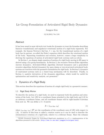
Lie Group Formulation of Articulated Rigid Body DynamicsJunggon Kim12/10/2012, Ver 2.01AbstractIt has been usual in most old-style text books for dynamics to treat the formulas describinglinear(or translational) and angular(or rotational) motion of a rigid body separately. Forexample, the famous Newton’s 2nd law, f ma, for the translational motion of a rigidbody has its partner, so-called the Euler’s equation which describes the rotational motionof the body. Separating translation and rotation, however, causes a huge complexity inderiving the equations of motion of articulated rigid body systems such as robots.In Section 1, an elegant single equation of motion of a rigid body moving in 3D space isderived using a Lie group formulation. In Section 2, the recursive Newton-Euler algorithm(inverse dynamics), Articulated-Body algorithm (forward dynamics) and a generalizedrecursive algorithm (hybrid dynamics) for open chains or tree-structured articulated bodysystems are rewritten with the geometric formulation for rigid body. In Section 3, dynamicsof constrained systems such as a closed loop mechanism will be described. Finally, inSection 4, analytic derivatives of the dynamics algorithms, which would be useful foroptimization and sensitivity analysis, are presented.11 Dynamics of a Rigid BodyThis section describes the equations of motion of a single rigid body in a geometric manner.1.1 Rigid Body MotionTo describe the motion of a rigid body, we need to represent both the position and orientation of the body. Let {B} be a coordinate frame attached to the rigid body and {A} bean arbitrary coordinate frame, and all coordinate frames will be right-handed Cartesianfrom now on. We can define a 3 3 matrixR [xab , yab , zab ](1)where xab , yab , zab 3 are the coordinates of the coordinate axes of {B} with respect to{A}. A matrix of this form is called a rotation matrix as it can be used to describe theorientation(or rotation) of a rigid body, relative to a reference frame. Since the columns1GEAR (Geometric Engine for Articulated Rigid-body simulation) is a C implementation of thealgorithms presented in this article. (http://www.cs.cmu.edu/ junggon/tools/gear.html)1
Figure 1: Coordinates frames for a rigid bodyof a rotation matrix are mutually orthonormal and the coordinate frame is right-handed,the rotation matrix has two properties,RRT RT R I,det R 1,(2)and it is denoted by SO(3)2 .Let p 3 be the position vector of the origin of {B} from the origin of {A}, andR SO(3) be the rotation matrix of {B} relative to {A}. The configuration space of therigid body motion can be represented with the pair (R, p), which is denoted as SE(3). A4 4 matrix, R p(3)T 0 1is called the homogeneous representation of T (R, p) SE(3), and its inverse can beobtained with TR RT p 1.(4)T 01From now on, a simple declaration, T SE(3) : {A} {B}, will be used to notify thatT SE(3) represents the orientation and position of a coordinate frame {B} with respectto another coordinate frame {A}.The Lie algebra of SE(3), denoted as se(3), is identified as a 6-dimensional vectorspace (w, v) 6 where w so(3), the Lie algebra of SO(3). ξ (w, v) se(3) can alsobe represented as a 4 4 matrix, [w] vξ (5)0 0 0 w3 w2where [w] w3 0 w1 3 3 is a skew-symmetric matrix. w2 w10The adjoint action of T SE(3) on ξ se(3), Ad : SE(3) se(3) se(3), is definedasAdT ξ T ξ T 1 .(6)2The notation SO abbreviates special orthogonal and ‘special’ refers to the fact that det R 1 ratherthan 1. See [2] for more details.2
From (3), (4) and (5), AdT can be regarded as a linear transformation, AdT : se(3) se(3), which is defined by a 6 6 matrix R0AdT (7)[p]R Rwhere T (R, p) SE(3). The coadjoint action of T on ξ dse(3) which is the dual ofξ, Ad T : dse(3) dse(3), is defined by a 6 6 matrixAd T AdTT.(8)1.2 Generalized Velocity and ForceLet T (t) (R(t), p(t)) SE(3) be a motion trajectory of a coordinate frame attached toa rigid body with respect to an inertial frame. The generalized velocity of the rigid bodyis defined as [w] v 1(9)V T Ṫ 0 0where [w] RT Ṙ and v RT ṗ. The physical meaning of w 3 is the rotational(or angular) velocity of the coordinate frame attached to the body relative to the inertial frame,but expressed in the body coordinate frame. Similarly, v 3 represents the velocity ofthe origin of the coordinate frame relative to the inertial frame, and still expressed in thebody frame. The generalized velocity is an element of se(3), and can be simply regardedas a 6-dimensional vector, i.e., wV .(10)vAs the generalized velocity is an instance of se(3), it follows the adjoint transformationrule defined in (7). Let {A}, {B} be two different coordinate frames attached to the samerigid body, and Ta , Tb SE(3) represent the orientation and position of the two frameswith respect to an inertial frame. Then, from (6) and (9), the generalized velocities of{A} and {B} have the following relation:Vb AdTba Va(11)where Tba SE(3) : {B} {A}.With a coordinate frame attached to a rigid body, the generalized force acting on thebody can be defined as mF (12)fwhere m 3 and f 3 represent a moment and force acting on the body respectively,viewed in the body frame. The generalized force is known as the member of dse(3), andhas the following transformation rule,Fb Ad Tab Fa(13)where Fa and Fb denote a generalized force viewed from different body frames {A} and{B}, and Tab SE(3) : {A} {B}.3
1.3 Generalized Inertia and MomentumThe kinetic energy of a rigid body is given by the following volume integralZ1e kvk2 dm2vol(14)which means the sum of the kinetic energies of all the mass particles constituting the body.By introducing a coordinate frame attached to the body, (14) can be restructured as thefollowing simple quadratic form,1e V T IV(15)2where V 6 is the generalized velocity of the body and I 6 6 , which is known asgeneralized inertia, represents the mass and mass distribution with respect to the bodyframe.To obtain an explicit form of the generalized inertia of a rigid body, let r 3 bethe position of a body point relative to the body frame and (R, p) SE(3) representsorientation and position of the body frame with respect to an inertial frame respectively.Using v 2 ṗ Ṙr 2 , RT Ṙ [w] and RT ṗ v, (14) can be rewritten asZ 1e (16) ṗ 2 2ṗT Ṙr Ṙr 2 dm2 vol Z Z Z1 ṗT ṗdm 2ṗT R[r]dm w wT[r]T [r]dm w(17)2volvolvol Z Z 1TTTT mv v 2v[r]dm w w[r] [r]dm w(18)2volvol1 V T IV(19)2where V (w, v) is the generalized velocity of the body and the generalized inertia, I,has the following explicit matrix form:#" RRTvol [r] [r]dmvol [r]dmI .(20)RT[r]dmm1volinertia is symmetric positive definite, and its upper diagonal term, I RThe generalizedT[r][r]dm,isthe definition of the well-known 3 3 inertia matrix of the rigid bodyvolwith respect to the body frame. If the origin of the body frame is located onR the center ofmass, then the generalized inertia becomes a block diagonal matrix because vol [r]dm 0.In addition, if the orientation of the body frame also coincides with the principle axes ofthe body, then the generalized inertia becomes a diagonal matrix.Let {A} and {B} be coordinate frames attached to a rigid body, Ia and Ib be thegeneralized inertias of the body corresponding to the two frames. Using (11), (15), andthe fact that the kinetic energy of the body should remain under change of coordinateframe, the following transformation rule between the generalized inertias can be obtained:Ib Ad Tab Ia AdTab4(21)
where Tab SE(3) : {A} {B}. If the mass, m, and the inertia matrix in a center ofmass frame3 , Ic 3 3 , are given, one can get the generalized inertia in an arbitrary bodyframe from (21), rather than using (20), as"#RIc RT m[p]T [p] m[p]I (22)m[p]Tm1where (R, p) SE(3) represents the orientation and position of the center of mass framewith respect to the body frame.The generalized momentum of a rigid body is defined asL IV(23)where I and V are the generalized inertia and velocity of the body expressed in a coordinate frame attached to the body.La and Lb be the generalized momentum of a rigid body expressed in different bodyframes, {A} and {B}, respectively. Using (11) and (21) one can derive the followingtransformation rule for generalized momentums:Lb Ad Tab La(24)which is same to that of generalized forces, and indeed, the generalized momentum is alsoknown as dse(3).1.4 Time Derivatives of se(3) and dse(3)PRecall that the time derivative of a 3-dimensional vector x 3i 1 xi êi , expressed in amoving coordinate frame {êi }, can be obtained as 3 Xdddx xi êi xiêi ẋ w x(25)dtdtdti 1 P3d1 dx2 dx3xi êi dx,,is the component-wise time derivative of xwhere ẋ i 1 dtdtdtdtand w is the angular velocity of the moving frame.The time derivatives of se(3) and dse(3) which are expressed in a moving frame havemore generalized form. A simple approach to obtain the derivatives is to transform se(3)(ordse(3)) to a stationary coordinate frame, differentiate it there, and transform the derivativeback to the original moving coordinate frame with the (correct) assumption that thederivative of se(3)(or dse(3)) can be transformed with the rule of se(3)(or dse(3)).4 Notethat differentiating a vector in a stationary coordinate frame with respect to time is justgetting the component-wise derivative of it.Lemma 1. Let X se(3) be expressed in a moving frame attached to a rigid body. Thenthe time derivative of X can be obtained bydX Ẋ adV Xdt3(26)A coordinate frame whose origin is located on the center of mass of the body.In [1] the time derivative of a spatial velocity which is similar to the generalized velocity in this articlewas obtained with this approach.45
where Ẋ is the component-wise time derivative of X and adV : se(3) se(3) is a lineartransformation defined as [w] 0adV (27)[v] [w]where V (w, v) se(3) is the generalized velocity of the body.Proof. Let T (R, p) SE(3) denote the orientation and position of the moving framewith respect to an inertial frame which is stationary in the space. By transforming X tothe inertial frame, differentiating it there, and then transforming the result back to theoriginal body frame, one can getdd0d0X AdT 1 (AdT X) Ẋ AdT 1 (AdT ) Xdtdtdt00ddwhere dtrepresents the component-wise differentiation and Ẋ dtX. Using (7) and0dTTV (w, v) (R Ṙ, R ṗ), one can show AdT 1 dt (AdT ) adV as follows: d0RT0Ṙ0AdT 1 AdT RT [p] RT [ṗ] R [p] Ṙ Ṙdt [w] 0 [v] [w]Lemma 2. Let Y dse(3) be expressed in a moving frame attached to a rigid body. Thenthe time derivative of Y can be obtained bydY Ẏ ad V Ydt(28)where Ẏ is the component-wise time derivative of Y and ad V : dse(3) dse(3) is a lineartransformation defined as T [w] 0 T(29)adV adV [v] [w]where V (w, v) se(3) is the generalized velocity of the body.Proof. Similarly to the proof of Lemma 1, the derivative of Y dse(3) can be obtainedby dd0d0Y Ad TAd T 1 Y Ẏ Ad TAd T 1 Y.dtdtdt0dUsing (8) and V (w, v) (RT Ṙ, RT ṗ), one can show Ad T dtAd T 1 ad V as follows: T 0R RT [p]Ṙ [ṗ] R [p] Ṙ d AdT AdT 1 0RT0Ṙdt [w] [v] adTV adV0 [w]6
1.5 Geometric Dynamics of a Rigid BodyEquations of motion of a rigid body can be written asF dLdt(30)where F represents the net sum of the generalized forces acting on the rigid body and Lis the generalized momentum of the body. Using (23) and (28), the equations of motionof the rigid body can be written asF I V̇ ad V IV(31)where V̇ is the component-wise time derivative of the generalized velocity of the body.Note that L̇ İV I V̇ I V̇ because the components of I doesn’t vary.The dynamics equation of a rigid body is coordinate invariant, i.e., the structure of theequation still remains under change of coordinate frame. Let {A} and {B} be coordinateframes attached to a body, Va and Vb be the generalized velocities, Fa and Fb be thegeneralized forces, and Ia and Ib be the generalized inertias corresponding to {A} and{B} respectively. Using the transformation rules, (11), (13), and (21), one can easilytransform the dynamics equations with respect to {A}, Fa Ia V a ad Va Ia Va , to theequations in {B}, Fb Ib V b ad Vb Ib Vb , and this shows the coordinate invariance of (31)under change of coordinate frame.2 Dynamics of Open Chain SystemsLet q n denote the set of coordinates of all joints in a system, and for open chainsystems, n is equal to the degree-of-freedom of the system. The dynamics equations ofthe system can be written asM q̈ b τ(32)where M (q) n n is a symmetric mass matrix of the system, b(q, q̇) n representsCoriolis, centrifugal, and gravity terms, and τ n denotes torque(or force) vector corresponding to the system coordinates q.We assume the current system state (q, q̇) is fully known. Calculating the joint torques(or forces for translational coordinates) τ with prescribe accelerations q̈ is called inversedynamics. It is typically used to obtain the required joint torques which make the systemmove along a prescribed joint trajectory. On the other hand, calculating the resulting jointaccelerations q̈ from the given joint torques τ is called forward dynamics, and this is usuallyused to simulate the system motion in time by integrating the computed acceleration toobtain the system state at the next time step.In general, the command input to a joint coordinate can be either torque or accelerationduring the simulation and the command type does not have to be same for all coordinates.Let’s rewrite the equations of motion as q̈uτuM b (33)q̈vτvwhere the subscript ‘u’ denotes the joint coordinates with prescribed acceleration andthe subscript ‘v’ represents the coordinates with given or known torque. We can obtain7
q̈ ττ q̈(q̈u , τv ) (τu , q̈v )Inverse dynamicsForward dynamicsHybrid dynamicsTable 1: Input and output of dynamics algorithms(τu , q̈v ) from the prescribed (q̈u , τv ) by solving the equations of motion, which is calledhybrid dynamics.5 One possible solution for hybrid dynamics is to rearrange (33) andsolve it with a direct matrix inversion. For example, the resulting accelerations of thetorque-specified joint coordinates can be obtained as 1q̈v Mvv(τv bv Muv q̈u )(34) uu Muv qubu,b where M MMuv Mvvbv , and q ( qv ). The method, however, is not efficient fora complex system because it requires building the mass matrix and inverting the submatrixcorresponding to the unprescribed joints, which leads to an O(n2 ) O(n3b ) algorithm wheren and nv denote the number of all coordinates and the number of unprescribed coordinatesrespectively.In Table 1 the input and output of inverse, forward, and hybrid dynamics are summarized. Note that hybrid dynamics is a generalization of traditional inverse and forwarddynamics, i.e., they can be regarded as the extreme cases of hybrid dynamics when qu q(inverse dynamics) and qv q (forward dynamics).2.1 Recursive Inverse DynamicsA recursive Newton-Euler inverse dynamics algorithm using the geometric notations shownin Section 1 was presented in [3]. Here the algorithm is slightly modified to support multidegree-of-freedom joints in the formulation.Let {0} be an inertial frame which is stationary in the space, {i} be a coordinate frameattached to the i-th rigid body of the open chain system, and {λ(i)} be a coordinate frameattached to the parent body of the i-th rigid body. Also, let Ti SE(3) : {0} {i},Tλ(i) SE(3) : {0} {λ(i)}, and Tλ(i),i SE(3) : {λ(i)} {i}. From Ti Tλ(i) Tλ(i),iand (6), the generalized velocity of the i-th body can be rewritten asVi Ti 1 Ṫi(35) 1 1 Tλ(i),iTλ(i)Ṫλ(i) Tλ(i),i Tλ(i) Ṫλ(i),i AdT 1 Vλ(i) Si q̇i (36)(37)λ(i),i 1where Si q̇i Tλ(i),iṪλ(i),i se(3) represents the relative velocity of the i-th body withrespect to its parent. Si Si (qi ) (se(3) ni ) is called the Jacobian of the jointconnecting the i-th body and its parent and qi ni represents the coordinate vector ofthe joint.As shown in (31), component-wise time derivatives of the generalized velocities of allbodies in the system are needed to build the dynamics equations for each body. Recalling5We follow [1] for the terminology.8
that Ȧ 1 A 1 ȦA 1 for an arbitrary matrix A, and adξ1 ξ2 ξ1 ξ2 ξ2 ξ1 for arbitrary ξ1 , ξ2 se(3), one can derive the following formula for V̇i , the component-wise timederivative of Vi : d0 1Tλ(i),i Vλ(i) Tλ(i),i Ṡi q̇i Si q̈idt 1 1 1 Tλ(i),iṪλ(i),i Tλ(i),iVλ(i) Tλ(i),i Tλ(i),iV̇λ(i) Tλ(i),iV̇i 1 Tλ(i),iVλ(i) Ṫλ(i),i Ṡi q̇i Si q̈i AdT 1 V̇λ(i) adAdλ(i),iVλ(i)T 1λ(i),i(38)(39)Si q̇i Ṡi q̇i Si q̈i AdT 1 V̇λ(i) adVi Si q̇i Ṡi q̇i Si q̈i(40)(41)λ(i),i(37) and (41) are well suited to calculate the generalized velocity and its componentwise time derivative of each body in a open chain system from the ground to the end ofthe system recursively, as the velocity and acceleration of the ground are known in mostcases.6 Note that Ṡi 6 0 as the joint Jacobian Si is a function of qi in general.Let Fi dse(3) be the generalized force transmitted to i-th body from its parentthrough the connecting joint, and Fiext dse(3) be a generalized force acting on the i-thbody from environment. Both Fi and Fiext are expressed in {i}. From (31), the equationsof motion for the i-th body can be written asXFi Fiext (42)Ad T 1 Fk Ii V̇i ad Vi Ii Vik µ(i)i,kwhere the left hand side of the equations represents the net force acting on the body,µ(i) is the set of child bodies of the i-th body, and Ad T 1 Fk is the generalized force,i,ktransmitted from k-th child body, expressed in {i}. It should be noted that the generalizedforce, Fi , for each body can be calculated by (42) from the ends to the ground recursively,as the end bodies have no child.A recursive inverse dynamics algorithm for open chain systems is shown in Table 2,and the following is a list of symbols for the geometric inverse dynamics: i index of the i-th body. λ(i) index of the parent body of the i-th body. µ(i) set of indexes of the child bodies of the i-th body. qi ni coordinates of the i-th joint which connects the i-th body with its parentbody. τi ni torque(or force) exerted by the i-th joint. Tλ(i),i SE(3) : {λ(i)} {i}, a function of qi . Vi se(3) the generalized velocity of the i-th body, viewed in the body frame {i}.6One can assume that V0 0 and V̇0 (0, g) where g 3 denote the gravity vector, viewed in theinertial frame, with appropriate direction and magnitude.9
V̇i se(3) component-wise time derivative of Vi . Si (se(3) ni ) Jacobian of Tλ(i),i viewed in {i}. 1 1 1 Tλ(i),i 1 Tλ(i),iSi Tλ(i),i q1 , · · · , Tλ(i),i qni , where qik denotes the k-th coordinate ofiithe i-th joint, i.e., qi (qi1 , · · · , qini ). Ii the generalized inertia of the i-th body, viewed in {i}. Fi dse(3) the generalized force transmitted to the i-th body from its parentthrough the connecting joint, viewed in {i}. Fiext dse(3) the generalized force acting on the i-th body from environment,viewed in {i}.Table 2: Recursive Inverse Dynamicswhile forward recursion doTλ(i),i function of qiVi AdT 1 Vλ(i) Si q̇iλ(i),iV̇i AdT 1 V̇λ(i) adVi Si q̇i Ṡi q̇i Si q̈iλ(i),iend whilewhile backward recursion doPFi Ii V̇i ad Vi Ii Vi Fiext k µ(i) Ad T 1 Fki,kτi SiT Fiend while2.2 Recursive Forward DynamicsFeatherstone [1] found that the dynamics equations of the i-th body can be reformulatedto have the following form,Fi Îi V̇i B̂i ,(43)where Îi is called as the articulated body inertia of the body and B̂i is an associatedbias force. He also showed that the articulated body inertia and bias force correspondingto each body in open chain systems can be calculated recursively, and by using thesenew quantities, forward dynamics can be solved with an O(n) algorithm. A Lie groupformulation of the articulated body inertia method was reported in [4]. Here, a moregeneral form of the geometric formulation supporting multi-degree-of-freedom joint modelsis presented.Starting from (43), we’ll show that the same form of dynamics equations still holds forthe parent of the i-th body(λ(i)-th body), and Îλ(i) and B̂λ(i) can be calculated from Îiand B̂i , which leads a backward recursion process for them.Let’s assume that the equations of motion for i-th body can be written as (43). By10
substituting (41) for V̇i in (43), one can get Fi Îi AdT 1 V̇λ(i) adVi Si q̇i Si q̈i Ṡi q̇i B̂i ,(44)and from SiT Fi τi , the unknown q̈i can be written as 1 q̈i SiT Îi Siτi SiT Îi AdT 1 V̇λ(i) adVi Si q̇i Ṡi q̇i SiT B̂i .(45)From (42) the dynamics equations for the λ(i)-th body becomesXextAd T 1 Fk ,Fλ(i) Iλ(i) V̇λ(i) ad Vλ(i) Iλ(i) Vλ(i) Fλ(i) (46)λ(i),iλ(i),ik µ(λ(i))λ(i),kand by substituting (44) for Fk in (46), one can getextFλ(i) Iλ(i) V̇λ(i) ad Vλ(i) Iλ(i) Vλ(i) Fλ(i) X AdT 1Îk AdT 1 V̇λ(i) adVk Sk q̇k Sk q̈k Ṡk q̇k B̂k .k µ(λ(i))(47)λ(i),kλ(i),kBy substituting (45) for the unknown q̈k in (47) and arranging the equations in terms ofV̇λ(i) , one can have the dynamics equations for the λ(i)-th body with the following desiredform:Fλ(i) Îλ(i) V̇λ(i) B̂λ(i)(48)whereÎλ(i) Iλ(i) Xk µ(λ(i))Ad T 1λ(i),k Îk Îk Sk SkT Îk Sk 1SkT Îk AdT 1λ(i),kextB̂λ(i) ad Vλ(i) Iλ(i) Vλ(i) Fλ(i) X Ad T 1B̂k Îk adVk Sk q̇k Ṡk q̇kk µ(λ(i))λ(i),k(49)(50) 1 Îk Sk SkT Îk Skτk SkT Îk (adVk Sk q̇k Ṡk q̇k ) SkT B̂k .In summary, the O(n) algorithm for forward dynamics of open chain systems consistsof the following three main recursion process:1. Forward recursion: recursively calculates Vi for each body with (37).2. Backward recursion: recursively calculates Îi and B̂i for each body with (49) and(50).3. Forward recursion: recursively calculates q̈i and V̇i for each body with (45) and (41).Table 3 shows the forward dynamics algorithm for open chain systems with a fewadditional intermediate variables, such as ηi , Ψi , Πi , and βi , for the simplicity and efficiencyof the equations.11
Table 3: Recursive Forward Dynamicswhile forward recursion doTλ(i),i function of qiVi AdT 1 Vλ(i) Si q̇iλ(i),iηi adVi Si q̇i Ṡi q̇iend whilewhile backward recursion doPÎi Ii k µ(i) Ad T 1 Πk AdT 1i,ki,kP extB̂i adVi Ii Vi Fi k µ(i) Ad T 1 βki,kΨi (SiT Îi Si ) 1Πi Îi ÎinSi Ψi SiT Îi oβi B̂i Îi ηi Si Ψi τi SiT Îi ηi B̂iend whilewhile forwardo do n recursionTq̈i Ψi τi Si Îi AdT 1 V̇λ(i) ηi SiT B̂iλ(i),iV̇i AdT 1 V̇λ(i) Si q̈i ηiλ(i),iFi Îi V̇i B̂iend while2.3 Recursive Hybrid DynamicsA geometric recursive algorithm for hybrid dynamics of open chain systems was reportedin [5], but the formulation was based on 1-dof joints. Here, more general form of thegeometric hybrid dynamics is presented to support multi-degree-of-freedom joints moreconveniently.One can derive the hybrid dynamics for open chain systems with a similar way as in2.2 for forward dynamics. Let’s go back to (47). Unlike the case of forward dynamics, asq̈k in (47) corresponding to an active joint is already known, one can arrange (47) in termsof V̇λ(i) by substituting (45) into (47) for q̈k of passive joints only as follows:Fλ(i) Îλ(i) V̇λ(i) B̂λ(i)12(51)
whereXÎλ(i) Iλ(i) Ad T 1 Îk AdT 1λ(i),kk {µ(λ(i)) u}X k {µ(λ(i)) v}Ad T 1λ(i),kλ(i),k Îk Îk Sk SkT Îk Sk 1SkT Îk(52) AdT 1λ(i),kextB̂λ(i) ad Vλ(i) Iλ(i) Vλ(i) Fλ(i) X AdT 1B̂k Îk adVk Sk q̇k Ṡk q̇k Sk q̈k λ(i),kk {µ(λ(i)) u}X λ(i),kk {µ(λ(i)) v} Îk Sk Ad T 1SkT Îk Sk 1 (53) B̂k Îk adVk Sk q̇k Ṡk q̇kτk SkT Îk (adVk Sk q̇k Ṡk q̇k ) SkT B̂k .where ‘u’ and ‘v’ denote the sets of the acceleration-prescribed and torque-specified jointsin the system respectively. Table 4 shows the hybrid dynamics algorithm for open chainsystems.Table 4: Recursive Hybrid Dynamicswhile forward recursion doTλ(i),i function of qiVi AdT 1 Vλ(i) Si q̇iλ(i),iηi adVi Si q̇i Ṡi q̇iend whilewhile backward recursion doPÎi Ii k µ(i) Ad T 1 Πk AdT 1i,ki,kPB̂i ad Vi Ii Vi Fiext k µ(i) Ad T 1 βki,kif i u thenΠi Îiβi B̂i Îi (ηi Si q̈i )elseΨi (SiT Îi Si ) 1Πi Îi ÎinSi Ψi SiT Îi βi B̂i Îi ηi Si Ψi τi SiT Îi ηi B̂iend ifend whilewhile forward recursion doif i u thenV̇i AdT 1 V̇λ(i) Si q̈i ηiλ(i),iFi Îi V̇i B̂iτi SiT Fi13 o
else on q̈i Ψi τi SiT Îi AdT 1 V̇λ(i) ηi SiT B̂iλ(i),iV̇i AdT 1 V̇λ(i) Si q̈i ηiλ(i),iFi Îi V̇i B̂iend ifend while3 Dynamics of Constrained SystemsLet q n denote a set of joint coordinates in an unconstrained open chain system, andA(q)q̇ 0 represents a set of m constraints enforced to the system (A m n ). Fora closed loop system, for example, a (virtual) unconstrained open chain system can beobtained by cutting the joint loops, and the closed loop constraints to be enforced can bewritten as f (q) 0, which can be linearized as the form of Aq̇ 0 where A f q is theJacobian matrix of the constraints.The equations of motion of the constrained system can be written as:M q̈ b τ AT λAq̇ 0(54)(55)where (54) represents the equations of motion of the unconstrained open chain system withan additional constraint force J T λ acting on the configuration space q, and the Lagrangemultipliers λ m give the relative magnitudes of the constraint forces.Similarly to the previous section (§2) we will derive inverse dynamics (q̈ τ ), forwarddynamics (τ q̈) and hybrid dynamics ((q̈u , τv ) (τu , q̈v )) for the constrained systemwhere q (qu , qv ). We assume the current system state (q, q̇) is known and consistentwith the constraints, and A is full rank.3.1 Inverse Dynamics of Constrained SystemsInverse dynamics finds the joint torques (τ ) satisfying the equations of motion when thecurrent system state (q, q̇) and the acceleration (q̈) are given. We assume the stateand prescribed acceleration (q, q̇, q̈) satisfy the constraints Aq̇ 0 and its differentialAq̈ Ȧq̇ 0, and focus on solving the equations of motion of the unconstrained systemwith the additional constraint force in (54).The inverse dynamics solution for a constrained system may not be unique dependingon the number of constraints and actuators. For example, when all joints can be actuated,any arbitrary constraint force λ and its corresponding joint torques τ M q̈ b AT λbecomes a solution of (54), and one particular solution is τ M q̈ b and λ 0 where thesystem acts as if it were a unconstrained open-loop system. In general, if the system isredundantly actuated or there are too many actuators, the joint torques that are requiredto make the system move in a prescribed way are not unique, and in this case, we oftenwant to choose an optimal one. On the contrary, if the number of actuators is fewer thanthe minimum necessary to move the system, there would be no solution as expected.14
Let q (qa , qp ) where qa and qp denote the actuated joint coordinates and non-actuatedor passive joint coordinates respectively. The passive joint torques τp need not to be zerobut they are assumed to be determined by the system state. We want to find the activejoint torques (τa ) satisfying (54) or τa ATτaraλ (56)τp ATτprpλwhere τr M q̈ b is the inverse dynamics solution for the unconstrained open chainsystem and the subscripts ‘a’ and ‘p’ denote the components for the active and passivecoordinates respectively and the subscript ‘r’ is for a solution of unconstrained dynamics.Since we already know τp , we can obtain the constraint force λ by solving the lower rowof (56) orAT(57)p λ τpr τp .If m np where m and np denote the numbers of constraints and the non-actuated 1coordinates respectively (Ap m np ), a unique solution λ AT(τpr τp ) exists7 .pFrom the upper row of (56), the active joint torques can be obtained as T 1τa τar AT(τpr τp ) .(58)a ApFor example, in a planar five-bar linkage system where the closed loop constrains twotranslation and one rotation axes (m 3), if there are two active joints (i.e., three of thefive joints are passive and np 3), we can obtain unique active joints from (58) as longas Ap is full rank or the configuration is not singular.However, if m np (e.g., a planar five-bar linkage with three or more active joints)8 ,there are infinite number of solutions for (57) which can be written as †λ AT(τpr τp ) N (AT(59)pp)where (·)† and N (·) denote the Moore-Penrose pseudoinverse and the null space of a matrixrespectively, and this leads to a general solution for the active joint torques as follows.τa τar ATaλno T †T τar ATA(τ τ) N(A)prpapp(60)(61)We can choose an optimal solution here: Constraint force minimization: †λ AT(τpr τp ).p The solution becomes τa τar ATa λ where Minimum active joint torques: We can find this by exploring the null space of ATpin (61). For example, in the case of n m np , o † n TT †τa 1 ATτar AT(τpr τp )(62)a N Aa Na Ap †λ AT(τpr τp ) N s (63)pno †T †s ATτar AT(τpr τp )(64)aNa Ap78We assume A is full rank.We call this a redundantly actuated system.15
minimizes kτa k2 where 1 na na denotes the identity matrix and N m (m np )np m . As a special case of this, if allrepresents a basis of the null space of ATp joints are actuated (n m, np 0), N becomes an identity matrix and thus theminimum joint torques and the corresponding constraint forces can be written asτ τr AT λ † 1λ AT τr AATAτr ,(65)(66)which can also be directly deduced from (56). In the case of n m, τa 0 becomesthe minimal torque solution, which means the system forms an immobile structuredue to too many constrain
Lie Group Formulation of Articulated Rigid Body Dynamics Junggon Kim 12/10/2012, Ver 2.01 Abstract It has been usual in most old-style text books for dynamics to treat the formulas describing linear(or translational) and angular(or rotational) motion of a rigid body separately. For example, the famous Newton's 2nd law, f ma, for the translational motion of a rigid body has its partner, so .