Transcription
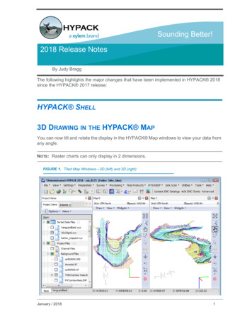
Sounding Better!2018 Release NotesBy Judy BraggThe following highlights the major changes that have been implemented in HYPACK 2018since the HYPACK 2017 release:HYPACK SHELL3D DRAWING IN THE HYPACK MAPYou can now tilt and rotate the display in the HYPACK Map windows to view your data fromany angle.NOTE: Raster charts can only display in 2 dimensions.FIGURE 1. Tiled Map Windows—2D (left) and 3D (right)January / 20181
Hand icon replaces the pan tool, to tilt and rotate the 3D display. Alternatively, you canuse keyboard controls: To tilt, Ctrl mouse wheel. To rotate, Shift mouse wheelThe angle of Rotation and Tilt appear in the Map status barTo adjust the scale of the Z axis, Shift Page Up and DownREMOTE TECHNICAL SUPPORT THROUGH BOMGARBomgar replaces TeamViewer to provide HYPACK Staff with remote access to yourcomputer for the purposes of technical support. The site is automatically launched from theRemote Assistance option in the Help menu. Contact HYPACK Support for a session key.The session key is a single, timed login for running remote support.PREPARATIONSOUND VELOCITYFIGURE 2. DownloadedSV DataPopulatesthe SOUNDVELOCITYProgram 2Valeport SWiFTSVP downloadinterfaces directlyvia Bluetoothconnections: SOUNDVELOCITYprogram: Whilethe SWiFT canexport aHYPACK *.VEL file fromthe ValeportDataLogsoftware, thisinterface makesit much easierfor you todownload the
SWiFT SVP sound velocity data directly into HYSWEEP SURVEY and theHYPACK SOUND VELOCITY program.Since the SWiFT SVP has a built in GPS, the SOUND VELOCITY program alsodownloads the time and position of the current cast. The position is displayed, in localcoordinates, based on the geodetic parameters in the current project. In HYSWEEP SURVEY, you must add the Valeport SWiFT SVP as a device in theHARDWARE program. You can then download the latest cast from the HYSWEEP SURVEY menu (TOOLS-VALEPORT SWIFT SVP CONTROL).Sound velocity is expressed in sounding units rather than always m/sec.HYPACK DRIVERS ADCP.dll: Support for DVL. Supports Rowe and Nortek devicesNEW! Autopilot.dll: Adds Quality Control messages from an Autonomous Vehicle. Includes a selection of alarms to alert you to possible data acquisition problems, andwhen the vehicle strays outside a user-defined area.Autolines.dll: Generates planned lines based on multibeam coverage.DVL.dll: Supports DVL without the ADCP driver. Uses Kalman to give better position thanthe ADCP driver.CMAX driver: Added pass through for magnetometer data.NEW! FLIRThermal.dll (FLIR) and Ladybugintf.dll (Ladybug 360) camera support toprovide photographic records of the survey site at user-defined intervals. Developed tocompare photos with topographic LiDAR data, MBMAX64 (64-bit HYSWEEP EDITOR)synchronizes the image display with the cursor position in based on the timestamp.You may also load Photos to the Project Items list to display a camera icon ateach image location in the Map window, then query the image to view the photoand its metadata.January / 20183
FIGURE 3. Images Captured using NEXUS Powered by HYPACK —JPG Properties Dialog (bottom left),Camera Icons in HYPACK Map (top right), ) 4Echologger.dll: Echogram support for EU D24 and EU400.LineOffset.dll: When you end line, the driver automatically creates next survey line at auser-defined distance along the normal of the previous survey line.Mavlink.dll: Controls unmanned vessels that follow the MavLink protocol.Navisound210.dll: Supports second transducer. Requires offsets for the second headand writes ECM records.Phins.dll: Separate records for heave, pitch and roll.Sontek M9 HS.dll: Set Lat/Long position in base stationNEW! SBG.dll: Support for PPS message to SBG inertial system.Subbot.dll: Ping Rate displays all changes in the rate. Synchronized with Discover. Resamples the long Ping Rate data to comply with SEG-Y specifications. Resamplingis maximum-based. Controls embedded in the main window. Supports multiple instances of subbot.dll in your HARDWARE configuration.TideDR shows both predicted and real-time tide in the graph.NEW! YSI Turbidity.dll: Checks turbidity levels every 2 minutes, displaying them on agraph, and can set an alarm if the level is above a threshold value.
HYSWEEP DRIVERSBathy NEW! Picotech sonarNEW! Norbit sonarR2Sonic added UHD modeReson Integrated dual head modeAncillary Devices NEW! Valeport SVP (via bluetooth)SBG: Added delayed heave supportGeneric Attitude: Added UDP option (added to serial)Additional devices pass GPS information through to HYPACK SURVEY. (Thisprovides single-cable operation as data is internally sent to SURVEY. RTA (Odom)POS (CeeScope)RRIO (ResonCV3 (OdomPingDSP Edgetech (6205)Edgetech –NMEAKongbergWASSPKlein HydroChartWater Column Support Reson compressed water column (7042)Teledyne MB2 water columnLiDAR NEW! Reigl VUX laser driverVelodyne driver added angle of beam (to beam number)Carlson Merlin name change from RenishawACQUISITIONRTCLOUDThe Real Time Cloud window provides a 3-dimensional display of your survey area.Originally developed for HYSWEEP SURVEY to merge hydrographic and topographicsoundings into one display, it is now also accessible from OPTIONS-SHARED MEMORY inHYPACK SURVEY and DREDGEPACK .Regardless of the project type, you may also provide further context to the point cloud displaywith the projection grid, charts and other project files (planned lines, plotting sheets, matrixfiles, etc.) displayed as charts.January / 20185
In HYSWEEP surveys, you may draw both hydrographic and topographic points in onedisplay. Alternatively, you could choose to draw your hydrographic data as a matrix, anddisplay only the topographic data in your point cloud.FIGURE 4. Real Time Cloud in a HYSWEEP SURVEYIn HYPACK SURVEY or DREDGEPACK , you can paint your matrix in the context of yourother project files in a 3-dimensional display.FIGURE 5. Real Time Cloud in DREDGEPACK (bottom)6
FIGURE 6. Real Time Cloud in HYPACK SURVEY (top) and DREDGEPACK (bottom)HYSWEEP Valeport SWiFT Support: Include the Valeport SWiFT SVP device in your HARDWAREconfiguration then download the most recent sound velocity profile, via Bluetoothconnection, directly to HYSWEEP SURVEY (TOOLS-VALEPORT SWiFT SVPCONTROL).RT Dual Head snippet display (dual head patch test). Choose which head paints thematrix in Survey when you are logging your patch test lines to assure coverage.The 64-bit HYSWEEP EDITOR synchronizes images with your survey data. Acamera icon appears in the Map window at each image position. Click an icon to see thecorresponding image displayed in a pop-up window.PROCESSING64-BIT SINGLE BEAM EDITORDevelopments in the SBMAX64 have continues as we strive to integrate all features thatwere available in the 32-bit version.January / 20187
ECHOGRAMThe Echogram Window provides an editable graphical display of analog data. It displays highfrequency (red) and low frequency (blue) depth data in a time vs distance graph (left) and thereturn strength information corresponding to the current cursor position (right). The windowsynchronizes with the other window displays, providing you with additional information andtools with which you may edit your data.FIGURE 7. Sample Echogram WindowFLOW VECTOR VIEWWhen you load raw SonTek M9 HydroSurveyor data, the 64-bit SINGLE BEAM EDITORautomatically loads the corresponding YDFF files and draws them in the Flow Vector window.The toolbar provides display and output options. 8Averaging samples: Average up to 100 samples to thin the data in the display.Vertical Range: Method options enable you to choose the vertical range included in thevector calculations.Display options include vector length and width, and the basis for coloring the voctors(direction, line, magnetic error or velocity). You may additionally include backgroundcharts for context and a legend to interpret the current colors.
FIGURE 8. Sample Flow Vector Window Output options: You can output flow vector data in any of the following formats: X, Y, Velocity text files: The data is saved with an XYZ extension, but the third valuein each record represents the velocity for the selected range.FIGURE 9. Spreadsheet Export 366 ********************************************* ***** ***** ***** *****-0.19 -0.01 0.01 -0.05 -0.02-0.11 -0.03 0.07 -0.07 0.03-0.08 0.00 0.06 -0.09 0.03-0.04 0.03 0.04 0.03 0.060.09 0.16 0.04 0.16 0.130.13 0.23 0.25 0.12 0.260.09 0.26 0.26 0.04 0.22Screen captures: Stored in BMP, TIF or PNG image format. These images are notgeo-referenced.Georeferenced CAD DXF files. Load them to HYPACK as a chart file or into a CADprogram.OVERLAYSYou can display up to three additional sounding files from the same survey line. The depthsare displayed according to the options set in the View Options and Color Settings dialogs.The overlaid data cannot be edited. It is only used as a reference, should you want tocompare the current data file to a previous survey of the same line.January / 20189
FIGURE 10. Overlays DialogYou can also display up to four channel templates inthe profile window. These are based on the templatesof the primary files.DEPTH INTERPOLATIONIf you remove sounding data, the data will beinterpolated or removed according to the status of theselection in the Settings dialog (EDIT-SETTINGS)which toggles between the two choices.If you have elected to interpolate, soundings will only be deleted if you remove data at eitherend of the survey line, rendering interpolation impossible.SMOOTHINGIf you have been surveying in rough waters and do not use a heave sensor, your data can bevery jagged. In cases such as these, you can smooth the position and depth of the correctedsoundings.10
FIGURE 11. Smooting Soundings—Before (left) and After (right)NOTE: This is not highly accurate. We recommend properly measuring heave, pitch and rollwith an MRU. This smoothing is only a close approximation.FILE INFORMATIONThe File Information report provides statistical data about the currently loaded data set.FIGURE 12. Sample File Information ReportFile InformationRec Count: 6235DepthMinimum: -1.994550Maximum: 54.058667DOLMinimum: -35.130744Maximum: 17.055726Tide CorrMinimum: -1.574800Maximum: 0.229658# SatsMinimum: 0Maximum: 10HDOPMinimum: 0.600000Maximum: 1.900000IMPROVED SPREADSHEET CONFIGURATION Double-click the Display Option items to add/remove them from the spreadsheet. It’squicker and easier than the arrow buttons!The current sounding is highlighted in yellow.January / 201811
FIGURE 13. SpreadsheetCLOUD Option to invert selection (EDIT-INVERT SELECTION).FIGURE 14. Inverting Selected Points (solid red)—Before (left) and After(right) 12Option to save deleted points to a separate XYZ file (FILE-SAVE DELETED TO XYZ).In Figure 14, we deleted the points on the end of each line (as in the “After” image) thensaved the results to Saved.xyz and the deleted points to Deleted.xyz. In Figure 15 we see(top to bottom) saved, deleted and both files displayed together.
FIGURE 15. Saved (top) , Deleted (center) and Both files (bottom)together show the two data sets fit exactlytogether to form the size and shape of the original data set in Figure 14 IMPORT-GEOTIFF menu item now also supports georeferenced PNG (Like thosefrom web maps) to color SOUNDINGS.Support for added third-party point cloud formats: Input: E57, LAS, LAZ, PTS, ASC Output: LAS, LAZ, PTSDATA CONVERTER (FORMERLY HSX CONVERTER) Same program, new name: The HSX CONVERTER title has been a misnomer for sometime. The program that began as the tool to convert third-party side scan formats to theHYPACK HSX format, has developed over time to support several other conversionsand file types. In 2018, the program, renamed DATA CONVERTER, still appears in theSide Scan menu, but also under UTILITES-FILE WORK.Supports Sonardyne *.SWF8 to HSX conversionSonTek YDFF to RAW file now includes GPS quality (QUA records) for RTK.Supports dual head Reson *.S7KHSX split by frequency. The program reads the information from the message in theheader and divides the data according to frequency. The output files append thefrequency to the rootname of the original file.January / 201813
SIDE SCAN TARGETING AND MOSAICKING New Angle Varied Gain option (Side Scan Ctrls, gain tab.The scale bar now includes the current cursor position in red at the bottom of theScan View display.24-BIT COLOR TABLEHYPACK 2018 offers two modes: 8-bit and 24-bit color depths. 8-bit mode is similar to the HYPACK 2017 mosaicking mode. This has, however, beenimproved to more fully utilize the 255 colors of the 8-bit color depth. You will notice moredetail in your mosaics, as well as a wider variety in colors.24-bit mode is completely new to TARGETING AND MOSAICKING for 2018. Using thismode makes over 16 million colors available for the mosaic, which provides increasedclarity, especially in areas with a similar signal return. The new mode generally takes 1.52 times longer to make a mosaic.CUSTOM COLOR PALETTESYou can neither modify the colors, nor the color distribution in the default color palettes thatcome in the HYPACK install; however, you can create or modify custom palettes for yourmosaic displays and output files in the Color Palette Editor. Custom palettes are savedseparately from your project, so you can use them across all of your side scan projects.In the Colors tab of the Side Scan Controls, click [Edit Custom Palettes] to open the ColorPalette Editor where you can load any existing palette and modify it by doing any of thefollowing: Adding or deleting colors (sliders)Choosing new colorsShifting color distributionTo save your palette, enter a name at the bottom right and click [Save Palette]. 14If you have modified a default palette, you must save your modifications to a newpalette. The editor suggests the name by appending (1) to the default palette name, butyou may change it. Your new palette appears in the Custom Palettes list.If you have modified a custom palette, you can overwrite the existing palette, or save itto a new palette with a different name.
FIGURE 16. Color Palette Editor—Default Gold (top), Custom Palette (bottom)IMAGE CAPTURE TARGET QUICK MARKThe Quick Mark method enables you to mark multiple target locations in quick succession,but there are no additional records about the target location. The program generates thetarget at the center of each user-defined area and stores JPG and Geo-TIF images of thearea, named with the timestamp of the targeted location, to the project \Side Scan Imagesfolder.FIGURE 17. Captured Images—JPG (left) , TIF on XYZ Soundings (right)January / 201815
SUB-BOTTOM PROCESSING Reads SEG, SEGY, SGY and Edgetech JSf. You can multiselect indiidual files or makeand load a catalog (*.LOG).Restores user-defined TVGIMPROVED SUPPORT FOR TARGETS Target Visibility Dialog: The Target Visibility dialog (REFLECTORS AND TARGETSTARGET VISIBILITY) controls which targets from the SBP target group appear in the subbottom profile display and, configured separately, in the View Tracks window.FIGURE 18. Target Visibility Dialog In addition, the Show Targets option in View Tracks tab of the Settings dialog toggles thedisplay of all targets in the group on and off. When you use this option, the column for thetracks window updates accordingly.These settings do not affect the targets displayed in the HYPACK area map.Target Properties: Source and Line Name properties are now captured with the Depth ofBurial attribute and stored with the target.FENCESThe sub-bottom fence diagram shows one or more profiles together in a 3-dimensional,interactive display. The options in the Settings dialog enable you to customize your display.Many of the SUB-BOTTOM PROCESSOR options are common to both the sub-bottomprofile and the fence diagram.16
FIGURE 19. Sample Fence Display—Layers Match on Intersecting LinesThe options in the Fences Diagram tab of the Settings affect only the Fence Diagram:FIGURE 20. Settings Dialog—Fences Diagram TabEXPORTING CORRECTED SOUNDINGSWhile you may record corrections to the RAW data file during acquisition, this data is notrecorded or applied to the SEG-Y files. In HYPACK , you must apply corrections to subbottom data in post-processing. (In addition, you can correct any layback and latency errors.)You can then export corrected All format (*.EDT) and XYZ data from the SUB-BOTTOMPROCESSOR.Past versions of the SUB-BOTTOM PROCESSOR included only sound velocity corrections.This year we’ve added tide corrections as well. EXPORT EDT options convert your digitized layers to All format files, one for each layer,and stores them in the project Edit folder. Additionally, it generates catalog files for eachexported layer.January / 201817
Tip: For further analysis, you can load the All format files to the HYPACK CROSSSECTIONS AND VOLUMES program. EXPORT XYZ options stores the digitized points to XYZ format files, one for each layer, inthe project Sort folder. You can choose to export depth, isopach or both as the Z-value.Each file is named with the format.DATA SPLITTER-JOINERThe DATA SPLITTER-JOINER is designed for you to define the segments of your RAW orHSX data that are useful for your survey and generate a new line set from the chosensegments. The program was initially designed convert long serpentine lines of unmannedvessel missions into a more conventional line file set removing the data on sharp turns and . Shows background files and other project files when you load your data. The programautomatically displays charts, matrix files, and border files that were enabled in the Shellwhen you opened the DATA SPLITTER-JOINER.Clip the original data tracks to a border file as an alternative to manually defining thelines with your cursor.Eliminates redundant data from any overlaps in the original data set.Show Sidescan Swath toggles a diagram of the data coverage in the Display window.FIGURE 21. DATA SPLITTER-JOINER—Main Window (left), Display Window (right), Output Results (bottom)18
2 Hand icon replaces the pan tool, to tilt and rotate the 3D display.Alternatively, you can use keyboard controls: To tilt, Ctrl mouse wheel. To rotate, Shift mouse wheel The angle of Rotation and Tilt appear in the Map status bar To adjust the scale of the Z axis, Shift Page Up and Down REMOTE TECHNICAL SUPPORT THROUGH BOMGAR Bomgar replaces TeamViewer to provide .