WIXLIB

ZaianeFurthermore, they find that trading volume increases andperformance decreases after going online.Chuang and Lee (2006) use data of US listed companies inthe period 1963-2001, to prove a variety of effects ofoverconfidence7 on financial markets. They confirm theassumption of Gervais and Odean (2001), that tradingprofits induce overconfident investors more frequently totrade. In addition, Chuang and Lee (2006) provide supportfor investors displaying a self attribution bias for highmarket volatility being due to the presence of investoroverconfidence, and for overconfident investors beingprone to trade more in relatively riskier securities, afterexperiencing market gains.Statman et al., (2006) test the market trading volumeprediction of formal overconfidence models using USmarket level. They find that monthly market turnover(proxy of trading volume), is positively related to laggedmarket returns. Vector autoregression and associatedimpulse response functions indicate that individual securityturnover is positively related to lagged market returns aswell as to lagged returns of the respective security. Kim andNofsinger (2007) confirm these findings using Japanesemarket level data. They identify stocks with varyingdegrees of individual ownership to test the hypothesis anddiscover higher monthly turnover in stocks held byindividual investors during the bull market in Japan.Griffin et al. (2007) investigate the dynamic relationbetween market wide trading activity and returns in 46countries. Many stock markets exhibit a strong positiverelation between turnover and past returns. This relation ismuch stronger for developing countries than for developedones. These findings hold when they control for volatility,alternative definitions of turnover, differing sampleperiods, and are present at both weekly and dailyfrequency. They find also that this relation is morestatistically and economically significant in countries withrestrictions on short sales, where corruption is higher, andwhere the allocative efficiency of the stock market isweaker. The return-volume relation is also stronger forindividual investors than for institutional or foreigninvestors.Chou and Wang (2011) examine a unique datasetobtained from the Taiwan Futures Exchange which recordsall account-level trades and orders. They differentiateempirically between overconfidence and disposition effectand demonstrate that different types of traders exhibitdifferent types and levels of behavioral biases.Lin (2011) utilizes the disposition coefficient to verifywhether the disposition effect exists in Taiwan and Chinesestock markets during the periods of financial crises, and todiscuss the differences of the disposition effect betweenappreciation and depreciation periods. The empiricalresults show that during the 1997 Asian financial crisis, thedisposition effect significantly exhibits in the both markets.On the other hand, during the 2008 global financial crisis,They characterize the overconfidence hypothesis by four testableimplications.7165the disposition effect only exhibits in Chinese stock market.Nevertheless, there are no significant differences ofdisposition effect between A-shares and B-shares.Prosad and al., (2013) find that biases like the dispositioneffect and overconfidence prevail in Indian equity marketand can lead to an increase in trading volume at marketlevel as well as at individual security level.HypothesisIn order to examine how trading activity relates to laggedreturns, we will test the following hypothesis:H1: Trading volume is positively related to lagged marketreturns.The positive trading volume response to lagged marketreturns is consistent with the overconfidence hypothesis. Infact, high market returns make investors overconfidentabout the precision of their private information. As a result,they trade more frequently which leads to high volume. Aswith Odean (1998) and Gervais and Odean (2001), wepredict a positive lead-lag relationship between pastmarket returns and trading volume.H2: Individual security turnover is positively related toboth lagged security and lagged market returns.The positive security trading volume response to ownlagged return is consistent with the disposition effect. Infact, the disposition effect indicates investors’ tendency toenjoy realizing gains on individual security and to defer thecombustion of losses (Shefrin and Statman, 1985). Wepredict a positive relationship between security trading andpast market returns.H3: Existence of a positive contemporaneous relationshipbetween trading volume and volatility.Large branch of theoretical and empirical research(Karpoff, 1987; Harris and Raviv, 1993; Shalen, 1993)relate volume to concurrent return volatility. We predict apositive contemporaneous relationship between tradingvolume and volatility.DATA AND METHODOLOGYOur database consists of monthly observations of ChineseShenzhen8 composite common stocks from January 2000 toDecember 20069. The data is obtained from Datastream. Wefocus on monthly observations under the perspective thatchanges in investor overconfidence occur over monthly orannual horizons (Odean, 1998b; Gervais and Odean, 2001;Statman et al., 2006). Following Lo and Wang (2000) andStatman et al., (2006), we measured trading activity withThe Shenzen Stock Exchange was established in April 1991. Thismarket exhibit strong growth in the past decade, and when combinedwith the Shangai Stock Exchange, are currently the ninth largest in theword (about 1,250 listed companies, with total market capitalizationexceeding 653.50 billion USD).9 We use monthly observations for trading volume and returns, but ourestimate of volatility is constrained by the availability of daily returns.8

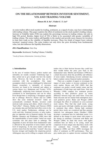
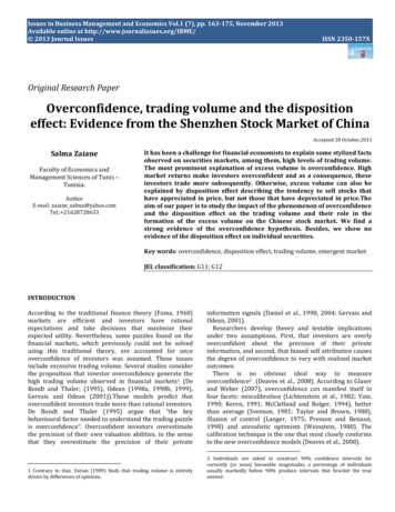
Issues Bus. Manag. Econ.166Volumecalculated as follow: Msig2 000001 6 11 16 21 26 31 36 41 46 51 56 61 66 71 76 81MonthsFigure 1: Monthly volume for Shenzhen compositeTTt 1t 1 r 2t 2 r t r t 1 , where rt isday t’s return and T is the number of trading days inmonth t; and this in order to adjust the first orderautocorrelation of returns. This volatility control variableis based on Karpoff’s (1987) survey of research oncontemporaneous volume–volatility relationship, as issimilar to the mean absolute deviation (MAD) measure inthe trading volume study of Bessembinder, Chan andSeguin (1996). According to French, Schwert andStambaugh (1987), non synchronous trading of securitiescauses daily portfolio returns to be autocorrelated,particularly at lag one10. However, the negative sign ofvariance in the case of some individual securities leads usTto use the approximation of Duffe (1995) (Msig2 r 2t ). Int 1fact, French, Schwert, and Stambaugh (1987)approximation results in a negative variance estimate ifthe first-order autocorrelation of daily returns in a givenmonth is (-0.5).Tutnover (%)21,510,5Summary statistics01 6 11 16 21 26 31 36 41 46 51 56 61 66 71 76 81MonthsFigure 2: Monthly turnover for Shenzhen composite marketturnover (shares traded divided by outstanding shares) andaggregate security turnover into market turnover on avalue-weighted rather than equal-weighted basis. We usealso another proxy (the volume), to measure the tradingvolume.Figure 1 and 2 present trading volume approximatedrespectively by volume (shares traded) and turnover, fromJanuary 2000 to December 2006. An examination of longterm Chinese trading volume indicates that the volume hasincreased over the last two years. The increase oftransactions can be explained by the existence of noisetraders.Definition of variablesMret : the monthly stock market return withdividendsmtrading : the monthly market turnover (sharestraded divided by outstanding shares) or the monthlyvolume (shares traded).msig : the monthly temporal volatility of marketreturn based on daily market returns within the month,correcting for realized autocorrelation, as specified inFrench, Schwert and Stambaugh (1987). The volatilityaccording to French, Schwert and Stambaugh (1987) isThe Table 1 provides summary statistics on monthlymarket return and market trading as well as a market-widebased control variable: volatility, during the period 20002006.To test for unit root, we employ the ADF and PhillipsPeron (PP test)11 for all variables. The test results12 indicatethat the null hypothesis that the variables are nonstationary is strongly rejected except for the variablesturnover and volume. Previous studies report strongevidence of both linear and non-linear time trend in tradingvolume series (Gallant et al., 1992; Chen et al., 2001).However, these linear time trend detrending methodologiesappear not flexible enough for time series (Statman et al.,2006). We employ the Hodrick-Prescott (1997) algorithm(HP) for detrending the trading variable13. In fact, the use ofnon stationary series can lead to bias in the coefficientstandard errors of vector autoregression we employ in thisstudy.Hodrick-Prescott (HP) algorithm is a two sided linearfilter that computes the smoothed series S of y byminimizing the variance of y around S, subject to a penaltythat constrains the second difference of S. Specifically, TheHP filter chooses St to minimize:See Fisher (1966) and Scholes and William (1977).A great advantage of PP test is that it is non-parametric, i.e. it does notrequire to select the level of serial correlation as in ADF. It rather takes thesame estimation scheme as in DF test, but corrects the statistic to conductfor autocorrelations and heteroscedasticity.12 For brevity tests of stationary are not reported.13 We use the natural log transformation before detrending the series.According to Statman et al. (2006), this can help eliminating thecorrelation between the level of the trend and volatility around the trend.1011

Zaiane167Table 1.Market descriptive 5402.60250.88520.6423MeanStd DevMinMaxSkewnessKurtosisJarque-BeraProb 32.21440.00001.09 E 161.19 E 164.13 E 165.08E 160.84293.11389.99270.0067 y t S t St 1 St St St 1 2t 1t 2T2T 1Detrended logturnover(mret)2.38 E-080.3776-0.80840 .98810.32222.49442.34850.3090(1)The penalty parameter , controls the smoothness of theseries St. The larger the , the smoother the St.As 14 , St approaches a linear trend. Our motivationfor detrending is to extract a stationary time-series, not topredict the trend15.To test the normality of returns, we refer toSkewness and Kurtosis statistics. For market return, theSkewness is 0 (0.77) and the Kurtosis is 3 (4.89). Thisimplies the non-normality of the distribution of returns.Empirical methodologyFollowing Statman et al., (2006) we use a vectorautoregression (VAR) and impulse response functions inorder to study the interaction between market returns andtrading proxies (turnover and volume).We use the following form of the VAR model:KYt a Ak Yt K Bl Xt l ek 1Ll 0t(2)where,Yt : a (nx1) vector of endogenous variables (returnand trading proxy : turnover and volume).Xt : a (nx1) vector of an exogenous variable :volatility.et : a (nx1) residual vector. It captures thecontemporaneous correlation between endogenousvariables.Ak : the matrix that measures how trading proxyand returns react to their lags.Bl : the matrix that measure how trading proxy andreturns react to month (t-1) realizations of the exogenousvariable.We follow the common practice of setting 14,400 for monthlyobservations.15 The detrended time series used in this study is the monthly differencebetween log trading and its trend.Detrended logvolume(mvol)3.57 0961.29054.592632.19650.0000K et L: numbers of endogenous and exogenousobservations. K and L are chosen based on the Akaike(1974) (AIC) and Schwartz (SC) information criteria16. Inour case, the SIC leads to K 517 and L 2. Glaser andWeber (2009) note that overconfidence models are notvery precise on how we should specify the lag length inempirical studies. Statman et al., (2006) find that returnsthat are lagged more than 6 months do not significantlyaffect trading activity anymore. Then, we employ impulseresponse functions to aggregate over coefficient estimatesand illustrate how the endogenous variables relate to eachother over time (Hamilton, 1994). Impulse responsefunctions trace the effect of a one standard deviation shockin one residual to current and future values of theendogenous variables through the dynamic structure of theVAR.Equation (3) contains two endogenous variables (marketturnover or market volume) and an exogenous variable(volatility): mtrading t mret t mtrading mret 5 mtrading t k Ak k 1 mrett k 2 msigt 1 emtrading, t (3) Bl l 0 emret, t Changes in one residual, say emtrading, t , will immediatelychange the current value of mtrading, but will also affectthe coefficient matrix of future values of mtrading and mretsince lagged values of mtrading appear in both equationsthrough the coefficient matrix AkTo test overconfidence, we shock the market return by onesample standard deviation and we track how markettrading activity responds over time to the market returnresidual.We introduce the market return (mret) in the VAR model ofindividual securities, in order to check if disposition effectexplains high trading volume as well as the overconfidence14Our choice is based on the Schwartz information criterion (SIC) (wechoose the number of lags which minimize the SIC).17 Chuang and Lee (2006) chose also 5 lags for their model.16

Issues Bus. Manag. Econ.168Table 2: Market VAR estimation (mtrading volume)Table 2.1. Relations with lagged market 2.22851] 0.13018)[0.17423]0.000752(0.00104)[0.72632]( ): Standard errors; [ ]: t stat; *: coefficient significant at the level of 5 %Table 2.2. Relations with lagged market (0.13626)[0.90315]( ): Standard errors; [ ]: t stat; *: coefficient significant at the level of 5 %hypothesis. For that, we use a trivariate VAR model for eachsecurity with 3 endogenous variables: security tradingvolume, market return and security return; and a singleexogenous variable, security volatility: trading it trading trading it k 6 2 ret Ak ret it kretBl sigtit l 0k 1 mrett mrett k mret l etrading, t eret,t emret, t (4)Where,tradingit : trading volume of the security i at montht;retit : return of the security i at month t ;Sigit : volatility of the security i at month t based onthe approximation of Duffe (1995).As with the model, we are concerned with how securitytrading response to shocks in returns, both security returnand market wide return. We introduce security return inorder to test the overconfidence predictions of Daniel et al.(1998). If overconfidence explains volume in addition todisposition effect, we should find a positive relationbetween past market return and security trading volumeeven when lagged security returns are introduced in themodel (Hypothesis 2).Market VAR estimation and test resultsMarket vector autoregressionTable (2) and (3) provide the results of equation (3). Thevariable mtrading in Table (2) represent volume. However,in Table (3), it represents turnover. The tables areorganised by rows for each endogenous variable (mret andmtrading) and by columns for lagged ones. For eachcoefficient, we report the estimated value, t statistic and thestandard errors.From the Table (2.1), we document that market trading isautocorrelated, with a significant one lag coefficients.However, Lagged observations of trading volume are notcorrelated to market return.The Table (2.2) presents the association between marketvolume and lagged market returns (hypothesis 1 of ourstudy). We remark that volume is positively related to lagmarket returns with only one significant coefficient (thefirst lag). This result is consistent with previous empiricalstudies of overconfidence hypothesis (Statman et al.(2006), Griffin et al. (2007), Chuang and Lee (2006) andGlaser and Weber (2007)). According to Glaser and Weber(2007) and Deaves et al. (2007), high market returns makethe investors overconfident in the sense that theyunderestimate the variance of stock returns. However,Hilary and Menzelt (2006) attribute this finding to the selfattribution bias. In fact, investors think that theirpredictions are better than the others.The Table (2.3) presents the relation betweenendogenous and the exogenous variable (msig). Results

Zaiane169Table 2.3. Relations with lagged (0.01361)[0.16248]( ): Standard errors; [ ]: t stat; *: coefficient significant at the level of 5 %Table 3. Market VAR estimation (mtrading turnover)Table 3.1.Relations with lagged market 85]mtradingt-3-0.051835(0.14032)[-0.36941]-3.24 E .040423(0.12776)[-0.31640]4.04 E 2735)[0.65575]0.130137(0.14683)[0.88632]( ): Standard errors; [ ]: t stat; *: coefficient significant at the level of 5 %Table 3.2. Relations with lagged market 1434(17.0482)[0.35613]0.147434(0.15382)[0.95849]( ): Standard errors; [ ]: t stat; *: coefficient significant at the level of 5 %show a positive and significant contemporaneousassociation between volume and volatility (Hypothesis 3).Our finding is consistent with Karpoff (1987) and Statmanet al. (2006)18. In Table (3), we replace volume by turnoveras a proxy of trading volume. We find the same results thanthose in Table (2). In fact, the relation between turnoverand lagged market returns is also significant with one lagsignificant coefficient. We still show a positive andsignificant contemporaneous association between volumeand volatility. However, market trading is notautocorrelated.Market impulse response functionsIndividual VAR coefficient estimates do not capture the fullimpact of an exogenous variable observation. An impulseIndividual coefficients on lagged msig must be interpreted with cautionbecause of autocorrelation in volatility (Gallant, Rossi and Tauchen, 1992;Chen, Firth and Rui, 2001).18response functions use all the VAR coefficient estimates totrace the full impact of a residual shock that is one samplestandard deviation from zero.Figure 3 contains all four possible impulse responsefunction graphs using the bivariate VAR estimation shownin Table (2) and (3). The vertical axis measures thepercentage increase in mtrading. We note that impulseresponse functions are forced to zero over time becausemtrading proxy is detrended.Figures (3.a) and (3.b) represent responses of mret to onestandard deviation of mret and mtrading along withconfidence bands spaced out at two standard errors. InFigure (3.a), the impulse response function indicates thatimpact of mret shock is positive and persistent for about 5months. Figure (3.b) indicates that a one standard deviationshock to mtrading increases slightly, but, in general, theimpulse response function coefficients are not significantlydifferent from zero.Figures (3.c) and (3.d) represent responses of mtradingto one standard deviation of mret and mtrading along w

stock returns and trading volume; it can potentially alter the previous findings of the developed markets (Pisedtasalasai and Gunasekarage, 2006).The goal of our paper is to study overconfidence and the disposition effect and their correlations with trading volume in the Chinese market.