WIXLIB

CHARNESS & GNEEZY: PORTFOLIO CHOICE AND RISK ATTITUDEStheir vague beliefs in situations where they feelparticularly knowledgeable or confident. Thus,perceived self-confidence or competence cantrump one’s aversion to ambiguity.Sarin and Weber (1993) test whether ambiguity aversion can survive market incentivesand feedback, using market experiments withsealed-bid and double-oral auctions andsophisticated subjects (graduate business students and bank executives). Each participantfaced both clear and vague bets about thecolor of a tennis ball to be drawn from anopaque urn, sometimes making both bets inthe same market and sometimes in differentmarkets. There is a pronounced decrease forindividual bids and market prices with lotteries featuring ambiguous probabilities relativeto bids and prices with lotteries where theseprobabilities are known. This effect was substantially stronger with the sealed-bid auctionmechanism, while the double-auction resultsare less compelling. Nevertheless, ambiguityaversion shows definite effects in a market setting with monetary incentives and feedback.Fox and Tversky (1995) test the relationship between risk and uncertainty using a seriesof studies involving Ellsberg’s two-color andthree-color problems, temperatures in nearand far cities, stock prices, and inflation rates.They note that previous tests had useda within-subject design in which participantscompared ambiguous and clear alternatives,and propose a comparative ignorance hypothesis. Both between-subject and within-subjectelicitation are used to test whether an awareness of missing information is per se sufficientto affect real bets with monetary incentives.The studies provide evidence that ambiguityaversion is ‘‘present in a comparative contextin which a person evaluates both clear andvague prospects, [but] . . . seems to disappearin a non-comparative context in which a person evaluates only one of these prospects inisolation.’’ This result will be important whenwe compare investment behavior of people ina noncomparative context.B. The Illusion of ControlLanger (1975) defines the illusion of controlas ‘‘an expectancy of a personal success probability inappropriately higher than the objective probability would warrant.’’ Langer findsthat choice, task familiarity, competition, and135active involvement all lead to inflated confidence beliefs. For example, Langer found thatpeople who were permitted to select their ownnumbers in a lottery game (hypothetically)demanded a higher price for their ticket thandid people who were assigned random numbers. Since this initial study, many otherresearchers have found that people often perceive more control than they actually have,make causal connections where none exist,and report surprisingly high anticipated predictive ability of chance events.3Presson and Benassi (1996) perform a metaanalysis of 53 experiments on the illusion ofcontrol and make a distinction between illusory control and illusory prediction. They findmuch greater effect sizes in experiments ‘‘thatmeasured participants’ perception of theirability to predict outcomes, as opposed to participants’ ability to control outcomes.’’ In fact,the authors point out (496): ‘‘Oddly enough,few experiments have actually measured illusory control in the sense that participantsjudge the extent to which they directly affectoutcomes.’’ Nevertheless, there is a sensethat some people do have some preferencefor direct control–for example, many crapsplayers care who rolls the dice at the table,and some strongly prefer to roll the dicethemselves.The predictive aspect of the illusion of control readily extends to the more general notionof overconfidence. In the behavioral financeliterature (e.g., Kyle and Wang 1997; Odean1999), an overconfident investor has historically been defined as one who overestimatesthe precision of his information signals.4 Overconfidence is most likely to manifest in environments with factors associated with skilland performance and some significant elements of chance.Two recent experimental studies investigateoverconfidence in investment behavior andemploy more direct measurement of overconfidence. Dittrich, Güth, and Maciejovsky (2001)allow participants to choose an investment3. Benassi et al. (1981, 25) find that ‘‘the introductionof objectively irrelevant factors (e.g., active involvement)into a chance task will lead people nevertheless to perceive(and behave as if) they can exert control over the task.’’4. An overconfident investor need not overestimatethe precision of all signals; for example, in the Daniel,Hirshleifer, and Subrahmanyam (1998) model, overconfidence is only present with respect to private informationsignals.

136ECONOMIC INQUIRYportfolio, and define overconfidence as theconsistently higher evaluation of one’s ownchoice over the optimal portfolio, as well asrisk-averse and risk-seeking portfolios. Theyfind that overconfidence increases with taskcomplexity and decreases with uncertainty.Biais et al. (2005) explicitly measure one’s disposition toward overconfidence by administering psychological tests and find thatoverconfident traders do tend to overestimatethe precision of their signals and earn relatively low profits in the accompanying experimental trading session.Nevertheless, none of the studies mentioned explicitly addresses the illusion of control, and to our knowledge this phenomenonhas not been tested in an investment experiment in which decisions are implemented withreal money. There are a number of reasonswhy an individual might be overconfident(e.g., a general predisposition or a belief specific to a particular situation), and we areinterested rather in the effect of direct participation in the process leading to a financialoutcome on the corresponding risk attitudesand portfolio choice. Our design accommodates both the control and prediction aspectsof the illusion of control.C. Myopic Loss AversionMyopic loss aversion (henceforth, ‘‘MLA’’)is a combination of two well-documentedbehavioral phenomena. The first is loss aversion, which is a major ingredient in prospect theory (Kahneman and Tversky 1979;Tversky and Kahneman 1992). According toprospect theory, the carrier of value is changerelative to a reference level. Loss aversion isthe tendency to weight negative changes fromthe reference level (losses) more heavily thanpositive changes (gains). The second phenomenon is mental accounting (Thaler 1985). Theaspect of mental accounting in play in relationto MLA is myopia, or the observation thatpeople tend to evaluate their investment portfolio frequently, even when the investment isfor the long run. Loss aversion combined witha tendency to focus on short-run outcomesgives MLA.To illustrate MLA, assume that the investment portfolio’s value follows a random walkwith a positive drift. Since people evaluatetheir portfolio frequently, they observe theshort-term losses (say from one period tothe other); because they are more sensitiveto losses than to gains, they are negativelyaffected by the short-term changes. Hence,the expected utility received from the portfoliois lower when the investor observes the frequent random changes.One of the most interesting puzzles infinance is the equity premium puzzle, first discussed by Mehra and Prescott (1985). Thispremium reflects the difference in returnsbetween equities (stocks) and risk-free assetssuch as government bonds or bills, and ithas historically been quite large. This puzzleis difficult to resolve within the standard neoclassical model; Benartzi and Thaler (1995)propose an explanation based on MLA.Thaler et al. (1997) and Gneezy and Potters(1997) use experimental designs in which thefrequency of the evaluation period (and opportunity to make investment choices) is varied. The shorter the evaluation period, thenoisier the asset price, and the more likely itis that a sale will result in a loss relative tothe most recently observed wealth level. Themain finding is that investors are more willingto invest a greater proportion of their portfolio in risky assets if they evaluate their investments less frequently; people who received themost frequent feedback took less risk andearned less money.5III. EXPERIMENTAL METHODWe conducted our experiments in classes atthe University of California at Santa Barbaraand the Graduate School of Business of theUniversity of Chicago. A total of 275 peoplewere involved in our sessions, with each person in exactly 1 of our 10 treatments. Wehanded out a one-page instructions/decisionsheet to the students in the class; these are presented in Appendix A. Every sheet had anidentification number written on two cornersof the page, and participants were instructed5. Two studies have attempted to delve further intowhether this phenomenon is driven by the informationfeedback or by decisions being binding for longer periodsof time. Langer and Weber (2001) replicate MLA whenboth features are present. However, Bellemare et al.(2004) find that decreasing the information feedback aloneleads to higher investment, while Langer and Weber(2004) find an increase in investment with restricted feedback. More research is needed to determine the interactionof the two influences.

CHARNESS & GNEEZY: PORTFOLIO CHOICE AND RISK ATTITUDESto tear off one of these corners. Each personwas confronted with a relatively straightforward decision task, deciding how much ofa 10 endowment to invest in a risky assetand how much to keep. Participants were toldthat 10% of the decision sheets would be chosen for actual implementation and payment.We drew numbers and matched these upwith the identification numbers on the decisionsheets to determine the investors chosen foractual payoff. Implementation of the investment instructions was done in private and theresulting earnings were paid in cash. Averageearnings follow from the average investmentpercentage in the risky asset. As this rate wasabout 70% overall, the average person selectedfor payment earned about 11.75.We now describe each treatment accordingto the phenomenon it investigates, and weidentify some predictions as given below.A. The Illusion of ControlWe had four different treatments in whichwe studied this issue. In all treatments, the rollof a six-sided die determines the value of therisky asset; the investor picks three ‘‘successnumbers’’; if any of these comes up, theamount invested pays 2.5 for every unitinvested. Allowing the participant to choose(or predict) winning numbers gives scope tothe predictive element of the illusion of control. The investor also chooses the numberof units to invest in the risky asset. In onetreatment (T2), the investor rolls the die; ina second treatment (T3), the experimenterrolls the die. In a third treatment (T1), theinvestor chooses who rolls the die, and neednot pay anything to get his or her wishes.Finally, in the fourth treatment (T7), theinvestor chooses the die-roller, but must pay5 units from the 100-unit allocation to personally roll the die. Thus, if we observe a preference to personally roll the die in T1, we wouldtest to see if this preference for control still persists at a cost.In a certain sense, T1 is the most attractiveoption since both those people who wish toroll the die and those people who want theexperimenter to roll the die get their wishesfreely. Thus, we might expect a higher investment rate in T1 than in T2 or T3. In addition,if there is a preference for control, more peoplepresumably get their wish in T2 than in T3, so137we might expect a higher investment rate inT2. Of course, the null hypothesis is thatinvestment is the same in each treatment.The predictions vis-à-vis T7 are less clear;although this is ex ante a less attractive optionthan T1, an investor who has already paidmoney to roll the die might feel the need to justify this expenditure by investing more heavily.B. Ambiguity AversionIn our next four treatments, the risky assetis successful if the investor correctly identifiesthe color of a marble that he or she will(blindly) draw from an opaque bag. In onetreatment (T5), there were 50 red marblesand 50 black marbles in the bag; in a secondtreatment (T6), there were 100 balls with anundisclosed distribution of red and black marbles. A third treatment (T4) mentioned bothbags and permitted the investor a free choicebetween them; in the fourth treatment (T8),this choice was also given, but it cost 5 unitsto choose from the bag with the known50-50 distribution of marbles.Here again, in a certain sense T4 is the mostattractive option since both those people wholike ambiguity and those people who dislikeambiguity get their wishes freely. Thus, wemight expect a higher investment rate in T4than in T5 or T6. In addition, if there is ambiguity aversion, people are presumably happierwith the lottery in T5 than in T6, so we mightexpect a higher investment rate in T5. Onceagain, the null hypothesis is that investmentis the same in each treatment, and the predictions across T4 and T8 are unclear.C. Myopic Loss AversionOur last two treatments examine the alternative evaluation periods used in Gneezy andPotters (1997).6 In the first treatment (T9), theinvestor chooses one of the two plans: (1) to beinformed of the value of the risky asset eachperiod and make allocations every period,or (2) to be informed of the value of the riskyasset after a block of three periods, and make6. Variations of this design were used to show theeffect of the investment horizon on market prices (Gneezy,Kapteyn, and Potters 2003), the possible negative effect ofemotions (Shiv et al. 2005), that teams are also prone tosuch influence (Sutter 2007), and that professional tradersare affected by the investment horizon even more thanstudents (Haigh and List 2005).

138ECONOMIC INQUIRYan investment choice for a block of three periods at a time. In the second treatment (T10),this same choice is offered, but every-periodinformation and investment opportunity costs5 units of each 100 units of endowment. In linewith previous studies, we might expect peoplewho choose to be informed each period in T9to invest more in the risky asset than peoplewho do not.FIGURE 1Preference for Control100755025IV. RESULTSWe find very different effects for the phenomena under consideration. In each case,people manifest a definite preference for onecondition. However, whether such preferencessurvive a price surcharge and whether theyaffect investment behavior varies considerablyaccording to the particular phenomenon. Ourfull data set is presented in Table A1.7A. The Illusion of ControlIn T1, people decide whether to roll the diethemselves or to have the experimenter roll thedie; in this treatment, there is no charge foreither choice. At the same time, the investorchooses what portion of his or her endowmentto invest in the risky asset. In T7, the setup isprecisely the same, except that it now costs 5%of the investor’s endowment for him or her toroll the die. In Figure 1, we show the percentage of participants who choose to roll the diein these two cases:When it is free to exercise a preference forcontrol, we find that 25 (68%) of 37 people inthis treatment chose to roll the die; if peoplewere indifferent, we should expect 50% choosing to roll themselves. The binomial test (Siegeland Castellan 1988) finds the proportionchoosing to roll is significantly different thanthe random prediction (Z 5 2.14, p 5 .016,one-tailed test). Thus, even a rather transparent illusion is enough to have a significanteffect on behavior. However, when it costs5% to exercise this preference, the proportionchoosing to roll drops dramatically—only 2 of7. We also collected information concerning gender,although we did not do so in some early sessions. Wesee a strong gender effect: On average, males invest75.27% and females invest 60.25%. A Wilcoxon ranksum test gives Z 5 4.52, p 5 .00000. This finding is discussed at length in Charness and Gneezy (2007).0Free to RollCostly to Roll22 (9%) people pay the price. This change inproportions is quite significant (Z 5 4.36,p 5 .00001) by the test of the difference of proportions (Glasnapp and Poggio 1985), so thatit seems that the preference for control is notvery deep or strong.If the illusion of control leads to greaterconfidence in successful outcomes, we shouldexpect a higher proportion to be invested inthe risky asset when the investor directly controls the outcome. Figure 2 shows the investment percentage in each of the four treatmentsregarding the illusion of control.We see very little variation across thesetreatments. When there is a free choice aboutrolling the die, the average proportioninvested in the risky asset is 70.6%. Whenthe investor rolls, this proportion is 70.5%,while when the monitor rolls this is 70.6%;there is a small increase to 73.5% when it costs5 units to roll the die. None of these proportions differ significantly, using the WilcoxonMann-Whitney rank sum test (Siegel andCastellan 1988). There is virtually no difference in the direct between-subjects test of investment percentage (investor rolls vs. monitorrolls). Restricting our attention to those treatments where people could choose who rolls thedie, we see very little difference in investmentpercentage between investors who chose toroll and who chose to have the experimenterroll. Pooling the data in T1 and T7, we findthat the proportions invested are 71.6% and71.9%, respectively. Thus, we cannot rejectthe null hypothesis of no difference in investment percentage, and the preference for control that we find does not appear to affectinvestment behavior.

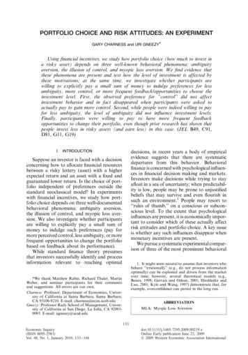
CHARNESS & GNEEZY: PORTFOLIO CHOICE AND RISK ATTITUDESFIGURE 2Investment % in Illusion RollsCostlyChoiceB. Ambiguity AversionIn our ambiguity aversion treatments, people chose a success color (red or black). In T4,they decide whether to select a ball from the bagwith the known 50/50 distribution or the bagwith an unknown distribution; there is nocharge for either choice. The investor alsochooses the portion of his or her endowmentto invest in the risky asset. In T8, the setupis precisely the same, except that it now costs5% of the investor’s endowment to select fromthe bag with the known distribution. Figure 3shows the proportion of people who prefer theknown distribution in these two cases:When it is free to choose from the bag withthe known distribution, 18 of 25 (72%) peoplechose to do so; this proportion is statisticallysignificant from randomness (Z 5 2.20, p 5.014, one-tailed binomial test), so that we haveevidence of ambiguity aversion. Charging 5%for indulging this preference reduced this proportion only slightly: 17 of 26 investors (65%)FIGURE 3Preference for Known Distribution1007550250FreeCostly139pay for the right to choose from the knowndistribution. This proportion is still marginally significantly different from randombehavior (Z 5 1.57, p 5 .058, one-tailed test),so that the preference for reduced ambiguitysurvives a modest cost; the difference betweenthe two observed proportions is not statistically significant (Z 5 0.51).If people feel that they have a greaterchance for success with less ambiguity or ifthey experience negative outcomes morekeenly with ambiguity, we might expecta higher proportion to be invested in the riskyasset when the investor chooses from theknown distribution. Figure 4 shows theinvestment percentage in each of the fourtreatments regarding ambiguity aversion:Once again, we see little variation acrossthese treatments. With free choice aboutknown or unknown distribution, the averageproportion invested in the risky asset is67.7%. When the distribution is known thisproportion is 64.0%, while with ambiguitythe proportion is 69.5%; there is again a smallincrease to 74.0% when getting a known distribution is costly. None of these proportions differ significantly (Z 5 0.88 for the comparisonbetween T5 and T8, the largest difference).Note that for the direct between-subjects comparison (ambiguous vs. known distribution),the slight difference in investment rates goesin the opposite direction from the prediction,and is in any case not statistically significant(Z 5 0.27).8 With ambiguity aversion, wedo find a difference in behavior in Treatments4 and 8 between investors who chose the knowndistribution and who chose the unknown distribution. Pooling these data, the proportionsinvested are 69.0% and 79.4%, respectively.However, this difference goes in the oppositedirection from the prediction! The test statistic8. It could be quite interesting to investigate whetherthere are differences in investment behavior in a withinsubjects test of ambiguity aversion. In line with the Foxand Tversky (1995) comparative ignorance hypothesisand the Sarin and Weber (1993) empirical support, wemight expect to see differential investment rates whenthe ambiguity is highlighted for each subject. This issueof relative evaluation is a relevant topic in marketingand business psychology, as Hsee et al. (1999) have shownthat people tend to make very different decisions depending on whether alternatives are evaluated separately ortogether. An additional treatment could be identical toTreatment 4, except that the investor would be told thata coin flip will determine whether he or she draws fromBag A or Bag B, and would be asked for investment decisions in each case.

140ECONOMIC INQUIRYFIGURE 5Preference for Every-Period PlanFIGURE 4Investment % in Amb

portfolio, and define overconfidence as the consistently higher evaluation of one's own choice over the optimal portfolio, as well as risk-averse and risk-seeking portfolios. They find that overconfidence increases with task complexity and decreases with uncertainty. Biais et al. (2005) explicitly measure one's dis-