WIXLIB

2power flow constraints might run into a local optimum andincorrectly declare robust feasibility while some infeasiblescenarios remain. Thus, to the best of our knowledge, no robustAC OPF solution algorithm that is guaranteed to satisfy eitheraspect has yet been published.We aim to develop an algorithm that addresses this gap. Asa first step, the AC OPF algorithm that is the main contribution of this paper focuses on the latter aspect of ensuringengineering constraint satisfaction for all realizations in aspecified uncertainty set. This is accomplished by formulatingthe robust AC OPF problem as a bi-level program where eachrobust constraint is replaced by a limit on the extreme valueachievable within the set of uncertainty realizations. Theseextreme values are obtained by solving a maximization (orminimization) problem over the uncertainty set, subject to ACpower flow constraints. To guarantee conservative estimatesof the extreme values, i.e., that the impact of uncertaintyis not underestimated, the power flow equations in the constraint maximization problems are replaced by a combinationof convex relaxations [15]–[21] (formulated as semidefiniteprograms (SDP) and second-order cone programs) that balancecomputational complexity with accuracy. Note that by applying the convex relaxations in this way, we guarantee feasibilityof the engineering constraints without any assumptions on therelaxation’s exactness or ability to find worst-case scenarios.To solve the resulting bi-level AC OPF problem, we adaptan alternating algorithm that has been successfully applied toother stochastic AC OPF problems [6], [7]. The algorithmalternates between 1) solving a deterministic, single-levelproblem with tightened constraint limits and 2) evaluatingan optimization problem for each engineering constraint tocompute constraint tightenings that ensure feasibility for alluncertainty realizations. The constraint tightenings’ dependence on the operating point (and vice versa) naturally leadsto an alternating algorithm. The algorithm has converged toa robustly feasible solution when the tightenings no longerchange between iterations.This paper is organized as follows. Section II describes howwe model uncertainty and the system’s response to disturbances. Section III formulates the robust AC OPF problem.Section IV details our iterative solution algorithm. Section Vprovides numerical results. Section VI concludes the paper.II. S YSTEM M ODELING UNDER U NCERTAINTYBased on typical system characteristics, this section presentsour models of the power system, the uncertain power injections, and the system’s response to fluctuations. Note that ourapproach can accommodate a range of variants in addition toour selected modeling choices.A. Notation and System ModelingWe consider a power system where N and L denote thesets of buses and lines, with N n. The set of buseswith uncertain demand or renewable generation is denoted byU N , and the set of conventional generators is representedby G. To simplify notation, we consider one conventionalgenerator, one composite uncertainty source, and one knowninjection per bus, such that G U N n. The network admittance matrix is denoted Y G jB, where j 1.Each bus i N has active and reactive power injections piand qi as well as a voltage phasor with magnitude vi andangle θi . To represent the steady-state behavior of typicalpower system devices, we use subscripts ( · )P Q , ( · )P V , and( · )θV to distinguish between PQ buses (specified active andreactive power injections), PV buses (specified active powerand voltage magnitude), and a single θV (specified voltagemagnitude and angle reference) bus. Each generator i G hasa quadratic cost function with coefficients c2,i , c1,i and c0,i .Each line ( , m) L has current flows into each terminali mv given by Ŷ m, where Ŷ m is the line’sim vmadmittance matrix. We use MATPOWER’s line model [22].B. Uncertainty ModelingThe active and reactive power injections at each bus i Nconsist of specified forecasted components, denoted as pinj,iand qinj,i , and fluctuations due to uncertain generation andload demand. Fluctuations in the active power injections,denoted as ω, belong to a specified uncertainty set W. Forsimplicity, we consider a box uncertainty set, i.e., each entry ofω lies within a pre-defined interval, ωi ωimin , ωimax whereωimin 0 ωimax . More general uncertainty sets (e.g., budgetuncertainty [23]) can also be modeled. Additionally, while thispaper does not explicitly consider voltage-dependent loads,extension to more general load models (e.g., ZIP models [24]and induction machine models [25]) is straightforward.We model the fluctuations as having constant power factorscos φi , such that the preactive power fluctuations are given by(1 cos2 φi )/ cos φi . Reactive powerγi ωi where γi could also be controlled in a variety of other ways, e.g.,as injections that are constant, dispatchable, or participate involtage control. These types of control can be included in theformulation without any conceptual changes.C. Generation and Voltage ControlSetpoints pG0 , qG0 , and vG0 for the active and reactivegeneration dispatches and voltage magnitudes are scheduledby the system operator based on the forecasted injections,corresponding to ω 0. During fluctuations ω 6 0, activepower deviations from the scheduled setpoints are determinedby an Automatic Generation Control (AGC) scheme [26]that dividesthe mismatch in total active power generationPΩ ωi U i among the generators accordingP to a vectorof prespecified participation factors α, where i G αi 1.While the deviation Ω due to uncertainty is the main sourceof power imbalance in the system, there is also an additionalpower mismatch due to changes in the active power losses.The total change in active power loss, denoted by δp, is alsosplit among the generators according to α such that the activepower generation is pG,i (ω) pG0,i αi (Ω δp).The reactive power outputs of generators at PV and reference buses, qG (ω), change to keep their voltage magnitudesconstant during fluctuations, whereas generators at PQ buseskeep their reactive outputs constant at qG0 . Conversely, the

3voltage magnitudes vG0 are kept constant by the generatorsat the reference and PV buses, but vary as functions of thefluctuations at PQ buses, v(ω).III. ROBUST O PTIMIZATION P ROBLEMThis section describes the robust AC OPF problem andexplains the problem’s challenges.A. Problem FormulationFormalizing the system and uncertainty models describedin Section II, the robust AC OPF problem isX minc2,i p2G0,i c1,i pG0,i c0,i(1a)of constraints. The requirement of robust feasibility in (1) canbe condensed into two key challenges:1) The power flow equations (1e)–(1g) must be guaranteedto have a solution for all uncertainty realizations ω W.2) No uncertainty realization ω W may result in violations of the engineering constraints (1h)–(1k).The remainder of this paper focuses on an algorithm foraddressing the latter challenge of preventing engineering constraint violations, with the task of rigorously addressing theformer challenge left as a subject for future work. To set up thedevelopment of our algorithm for ensuring engineering constraint satisfaction, we reformulate (1) as a bi-level program:mini Gsubject to ( i N , ( , m) L, ω ! W)XpG,i (ω) pG0,i αi(ωi ) δp(ω) ,(1b) j {NP V , NθV } ,(1c) k NP Q ,(1d)nh Xvk (ω) Gik cos θi (ω)pG,i (ω) pinj,i ωi vi (ω) k 1 i θk (ω) Bik sin θi (ω) θk (ω) ,(1e)nh XqG,i (ω) qinj,i γi ωi vi (ω)vk (ω) Gik sin θi (ω)k 1 i θk (ω) Bik cos θi (ω) θk (ω) ,(1f)vj (ω) vG0,j ,qk (ω) qG0,k ,θθV (ω) 0,(1g)maxpminG,i pG,i (ω) pG,i ,(1h)max qG,i (ω) qG,i,max vi (ω) vi , i m (ω) imax m , im (ω) (1i) imax m .c2,i p2G0,i c1,i pG0,i c0,i (2a)i Gi UminqG,iviminX(1j)(1k)The objective (1a) minimizes the cost of the scheduled activepower generation. Constraints (1b)–(1d) model the generators’responses to fluctuations ω 6 0 as described in Section II-C.The power flow equations (1e) and (1f) enforce power balancefor all uncertainty realizations. Constraint (1g) sets the anglereference. The generation constraints (1h) and (1i) limit thegenerator power outputs, while (1j) keeps the voltage magnitudes within bounds. The transmission constraints (1k) limitthe magnitudes of the current flows on every line.The variables in (1) can be classified into two categories:1) control variables pG0 , qG0 , and vG0 which representscheduled setpoints determined by the optimization problemand 2) dependent variables pG (ω), qG (ω), vG (ω), θ(ω), i(ω),and δp(ω) which are implicitly determined by the controlmodel (1b)–(1d) and the power flow equations (1e)–(1g) forall uncertainty realizations ω W.B. Discussion of ChallengesThe robust AC OPF problem (1) is a semi-infinite programsince the constraints must be satisfied for all realizations withinthe continuous uncertainty set W. Developing a tractablerepresentation requires reformulating (1) to obtain a finite setsubject to ( i N , ( , m) L, ω W) ,Constraints (1e)–(1g) for all ω W,(2b)(2c)min {pG,i (ω) s.t. (1b)–(1g), v(ω) v} pminG,i , max {pG,i (ω) s.t. (1b)–(1g), v(ω) v} pmax(2d)G,i ,ω W minmin {qG,i (ω) s.t. (1b)–(1g), v(ω) v} qG,i ,(2e)ω W maxmax {qG,i (ω) s.t. (1b)–(1g), v(ω) v} qG,i,(2f)ω W min {vi (ω) s.t. (1b)–(1g), v(ω) v} vimin ,(2g)ω W max {vi (ω) s.t. (1b)–(1g), v(ω) v} vimax ,(2h)ω W max { i m (ω) s.t. (1b)–(1g), v(ω) v} imax(2i) m ,ω W max { im (ω) s.t. (1b)–(1g), v(ω) v} imax(2j) m .ω W The first challenge of ensuring power flow feasibility is evidentby the presence of constraints (1e)–(1g) in (2b). The secondchallenge of guaranteeing the satisfaction of the engineering constraints for all uncertainty realizations appears in thesubproblems in (2c)–(2j). The formulation requires that eachconstraint is enforced for the ω that maximizes (or minimizes)the respective constraint value, which guarantees feasibility ofeach separate constraint for all ω W.Note that the optimization problems in (2c)–(2j) followthe generation and voltage control model (1b)–(1d) and thepower flow constraints (1e)–(1g), and include a lower boundon the voltage magnitude v. The lower bound v is selected to be significantly below practical operating regimes,e.g.,0.5 per unit (p.u.). This bound precludes the possibility ofundesirable “low-voltage” solutions in the absence of otherengineering constraints (which are not enforced to avoidcircular arguments).1 Imposing this bound is not restrictivein practice since the system model is invalid for very lowvoltages due to under-voltage protection schemes that woulddisconnect loads and generators prior to reaching such lowvoltage magnitudes.ω W1 When feasible, the power flow equations (1e)–(1g) are typically satisfiedby one “high-voltage” solution with near-nominal voltage magnitudes andpossibly many “low-voltage” solutions. These low-voltage solutions are undesirable since they are generally unstable and typically violate engineeringconstraints (1h)–(1k). Since we do not enforce (1h)–(1k) in the subproblems (2c)–(2j), imposing a lower bound of v screens out these solutions to avoid unnecessary conservatism that would resultfrom considering them.

4IV. A N A LGORITHM E NSURING ROBUST F EASIBILITY OFTHE E NGINEERING C ONSTRAINTSThe robust AC OPF problem requires that the engineeringconstraints (1h)–(1k) are satisfied for all possible uncertaintyrealizations ω W. This section explains our algorithm forenforcing these constraints in three steps. First, we describeour procedure for evaluating each individual constraint ata given scheduled operating point pG,0 , qG,0 , vG,0 . Next,we use our constraint evaluation procedure to represent therobust AC OPF problem as a deterministic AC OPF problemwith tightened constraints. Finally, we present our alternatingalgorithm that leverages the prior two steps to find an operating point that ensures robust feasibility of the engineeringconstraints.A. Evaluation of the Robust Feasibility ConstraintsThe optimization problems (2c)–(2j) maximize (or minimize) the constraint value with ω W as an optimizationvariable, subject to our uncertainty response model governingthe balancing behavior of generators and the AC power flowequations. Since the AC power flow equations are non-convex,the optimization problems may return a locally optimal solution that underestimates the impact of uncertainty. Therefore,we replace the non-convex problems (2c)–(2j) with convexrelaxations that are guaranteed to return conservative boundson the worst-case uncertainty impacts. While any relaxationis acceptable, we specifically use a combination of the sparseSDP relaxation [15]–[17] and the QC relaxation [18] alongwith a variety of improvements [19]–[21]. This choice ofrelaxations balances computational complexity with tightnessin order to avoid overly conservative solutions (i.e., that theimpacts of uncertainty are significantly overestimated due tothe use of relaxations that are too loose).The QC relaxation [18] requires specified angle differenceminmaxlimits θ m θ (ω) θm (ω) θ m, ( , m) L, satisfying minmax 90 θ m θ m 90 . We impose these limits in (2c)–(2j). Thus, our implementation implicitly assumes that nouncertainty realization results in very large angle differences.Similar to the assumed prohibition of unreasonably smallvoltage magnitudes in Sections III, we choose extreme valuesmaxminfor θ mand θ m, e.g., 60 , in order to avoid eliminatingrelevant portions of the subproblems’ feasible spaces.We iteratively solve the optimization problems:Step 1–Initialization: Solve relaxations of all optimizationproblems (2c)–(2j) as well as similar problems for the angledifferences θ ,m (ω) θ (ω) θm (ω) in order to obtaininitial bounds on pG (ω), qG (ω), v(ω), i(ω), and θ ,m (ω).Step 2–Iterative Tightening: The tighter bounds on pG (ω),qG (ω), v(ω), i(ω), and θ ,m (ω) from the previous iteration facilitate the construction of tighter relaxations. Usingthese tighter relaxations, we again solve relaxed versionsof (2c)–(2j) and the problems associated with the angledifferences.Similar to “bound tighening” techniques [19], [20], we repeatstep 2 until the relaxations cannot be tightened further.Note that the bounds on the voltage magnitudes v(ω) andthe angle differences θ ,m (ω) resulting from this iterativeprocess are typically substantially tighter than the initiallyminimposed limits, v and θ m, θmax . This suggests that that our v(ω) v mminmaxinitial assumptionsand θ m θ ,m (ω) θ m not restrictare sufficiently mild, and dothe feasible spacesof (2c)–(2j).B. Representation as Tightened ConstraintsAfter evaluating the robust constraints, we compute thedifference between the worst-case values and the values for agiven scheduled operating point. For active power, this yieldsλpmax max {pG,i (ω) s.t. (1b)–(1g), v(ω) v} pG0,i ,G,iω W (3a)λpmin pG0,i min {pG,i (ω) s.t. (1b)–(1g), v(ω) v}G,iω W (3b)By definition, λpmaxand λpminare non-negative and representG,iG,ithe range within which the corresponding value might vary.max , λ min , λv max , λ min , λiAnalogous values λqG,i, andqG,ivi miλim , i N and ( , m) L, are computed for allconstraints.The robust constraints (2c)–(2j) are tighter than the corresponding deterministic constraints, i.e., considering robustfeasibility shrinks the feasible space. As a consequence, λ 0,and one can interpret λ as providing constraint tighteningsthat account for uncertainty. We use this interpretation toreformulate (2) asX minc2,i p2G0,i c1,i pG0,i c0,i(4a)i Gsubject to ( i N , ( , m) L)Constraints (1e)–(1g) for ω 0,(4b)pmin pG0,i pmax,G,i λpminG,i λpmaxG,iG,i(4c)minqG,i(4d)viminmin qG0,i λqG,i λvimin v0,i i0, m i0,m imax mimax m λi m , λim .maxqG,ivimaxmax , λqG,i λvimax ,(4e)(4f)(4g)where pG0 , qG0 , v0,i , i0, m , and i0,m denote the generatoroutputs, voltage magnitudes, and current flows correspondingto the scheduled operating point, rather than being functions ofthe uncertainty realizations ω. Note that (4) is not equivalentto (2) since the AC power flow constraints (4b) are enforcedonly for the scheduled operating point, i.e., (4b) only considersω 0 rather than ensuring power flow solvability for allω W. This reformulation reduces the optimization problemfrom a semi-infinite program to a problem with a finite set ofconstraints. Under the assumption that power flow solvabilityfor all uncertainty realizations (i.e., existence of a solutionto (4b) for all ω W) is implied by feasibility of theengineering constraints for all ω W and satisfaction of theAC power flow equations at the scheduled operating point,a solution to (4) guarantees robust feasibility for the originalproblem (2). Although we expect this assumption to hold for

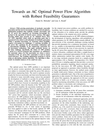
5Initialize: k 0 and constraint tightenings λ̂0 0k k 1 i4,2 (p.u.)Compute constraint tightenings:kkλ̂k 1 λ(pkG0 , qG0, vG0) 32100.62Solve deterministic, single-level AC OPF:kkpkG0 , qG0, vG0 arg min (4)with specified tightenings λ̂kOriginalLimit0.6 3200 3190 31800.58TightenedLimit 3170 31600.56 3150Check convergence:Is max( λ̂k 1 λ̂k ) η ?0.54No 31400.38YesConverged to a secure operating point!0.40.420.440.460.480.5 i4,1 (p.u.)(a) Feasible space for the deterministic AC OPF problem.Fig. 1. Alternating algorithm for robust AC OPF problems.C. Algorithm DescriptionFig. 1 summarizes our algorithm for solving (4). Thisalgorithm (which is similar to an algorithm previously appliedto chance-constrained AC OPF in [6], [7]) alternates between1) solving a deterministic, single-level AC OPF problem basedkon a given set of constraint tightenings, λ̂ , to obtain a solutionkk, vG0at iteration k, and 2) computing the constraintpkG0 , qG0tightenings λ̂k 1 for this solution by evaluating (3) for eachconstraint. The algorithm is initialized with λ̂0 0, suchthat the first iteration solves the deterministic, single-levelproblem associated with the forecasted values (ω 0). Forthe deterministic, single-level AC OPF problems (4) solvedin each iteration, any solution algorithm can be applied. Thealgorithm converges when the changes in the constraint tightenings between subsequent iterations are within a specifiedthreshold η 0, i.e., λ̂k 1 λ̂k η.While this algorithm may fail to converge or yield a suboptimal solution, it has been observed to perform well forother AC OPF problems under uncertainty, such as chanceconstrained AC OPF [6], [7], and the empirical results discussed in the following section are promising.V. N UMERICAL R ESULTSA. ImplementationThe algorithm is implemented using MATPOWER [22] tosolve the deterministic AC OPF problem in each iteration. The0.62 i4,2 (p.u.)many practical systems, providing more rigorous guaranteesregarding power flow solvability is an important aspect of ourongoing work.Reformulating problem (2) as (4) does not directly indicatea viable solution algorithm since the tightenings λ do nothave explicit representations. However, as described above,computing appropriate tightenings λ for a given scheduledoperating point pG0 , qG0 , vG0 is tractable. Moreover, theoptimization problem (4) is a tractable deterministic, singlelevel problem if the values of the tightenings λ are specified.We next present an algorithm that exploits these observationsto ensure robust feasibility of the engineering 0.540.380.40.420.440.460.480.5 i4,1 (p.u.)(b) Uncertainty realizations.Fig. 2. Projections of the feasible space and uncertainty realizations forcase6ww.computation of the tightenings using the relaxations in [15]–[21] is implemented in Matlab and YALMIP [27] with Mosekas a solver. We choose equal participation factors αi 1/ G , i G. In our experiments, the algorithm typically convergesin two to five iterations. For small systems, such as the 6bus system “case6ww” and the IEEE 14-bus system [22], asolution is obtained within two minutes on a laptop with aquad-core 2.70 GHz processor and 16 GB of RAM. Largersystems, such as the IEEE 30-bus or EPRI 39-bus systems,had solution times on the order of 10 to 20 minutes. Ratherthan being inherent to the algorithm, these solution timesare a rough indication of complexity. There are several waysof significantly improving computational speed, particularlyby reducing the time required to compute the constrainttightenings. Improving computational speed is an importanttopic for future work.B. 6-Bus Illustrative ExampleFig. 2 illustrates algorithmic performance using the 6-bussystem “case6ww” from [22]. The uncertainty set consideredfor this example is 5% variation around the forecasted valueat every load bus. The algorithm converges in three iterations.1) Impact of Robustness on AC OPF Solution: The coloredregion in Fig. 2a is a projection of the feasible space for the

6Alternating AlgorithmPG (MW)QG (MVAr)97.2419.2156.1671.0364.0588.45“case6ww” system computed using the approach in [28]. Theregion surrounded by the blue dashed curve corresponds to thefeasible space of the deterministic AC OPF problem solved inthe final iteration of the alternating algorithm. The solid blackline indicates the original deterministic limit on the line flowi4,2 while the dashed black line indicates the tightened flowlimit. The red square and blue star correspond to the solutionof the original deterministic AC OPF problem and the robustsolution based on the alternating algorithm, respectively.The robust algorithm introduces non-zero constraint tightenings λ to account for the impact of uncertainty, hencereducing the feasible space of the deterministic problem (4)that optimizes the operating point for ω 0. This results in1.2% higher operating cost for the robust operating point (bluestar) relative to the solution without considering uncertainty(red square). Table I compares the generator outputs for thesolution to the original deterministic AC OPF problem and theresult of the alternating algorithm. Ensuring robustness resultsin substantially different operation for this test case.2) Evaluation of Robust Feasibility: Fig. 2b shows theoperating points corresponding to 1000 randomly sampled uncertainty realizations based on the solutions from the originaldeterministic AC OPF problem (red) and the robust algorithm(blue). While many of the red dots indicate violations ofthe operational limit on i4,2 (i.e., they are above the currentlimit indicated by the black line), all uncertainty realizationsassociated with the output of the alternating algorithm resultin feasible operation (remain below the black line). This resultshows the robustness of the solution from our algorithm.The yellow triangles in Fig. 2b correspond to points wherethe SDP relaxation used in the last iteration of the alternatingalgorithm is exact and therefore yields a physically meaningfulextreme uncertainty realization. In particular, the SDP relaxations associated with maximizing current flow magnitudesare exact. As a result, the corresponding yellow triangles areat the extrema of the uncertainty realizations denoted by theblue dots. If the relaxations for these constraints had not beenexact, the strict bounds resulting from the relaxations wouldyield tighter constraints and thus a more conservative operatingpoint (i.e., the feasible space enclosed by the blue dashed linein Fig. 2a would shrink, and the largest uncertainty realizationsin Fig. 2b would shift down, away from the limit).C. IEEE 14-Bus SystemWe next present results for the IEEE 14-bus system [29]with 1 to 30% variation relative to the forecast for everyload. We reduce the line flow limits to 25% of the nominalvalues specified in [29] to obtain interesting behavior.1) The Impact of Uncertainty on Cost: Fig. 3 shows thecost of the robust AC OPF solution for varying levels of1.061.04

Even deterministic AC OPF problems are non-convex and generally NP-Hard [1], [2]. A wide variety of algorithms have been applied in order to find locally optimal AC OPF solutions [3]. Recent efforts have provided a broad range of "convex relaxation" techniques for AC OPF problems, which replace the AC power flow constraints by a convex outer