Transcription
Optimal Power Cost Management Using Stored Energy inData CentersRahul Urgaonkar, Bhuvan Urgaonkar†, Michael J. Neely‡, Anand Sivasubramaniam†Advanced Networking Dept., Dept. of CSE†, Dept. of EE‡Raytheon BBN Technologies, The Pennsylvania State University†, University of Southern California‡Cambridge MA, University Park PA†, Los Angeles CA‡rahul@bbn.com, {bhuvan,anand}@cse.psu.edu† , mjneely@usc.edu‡ABSTRACTCategories and Subject DescriptorsC.4 [Performance of Systems]: Modeling techniques; Design studiesGeneral TermsAlgorithms, Performance, TheoryKeywordsPower Management, Data Centers, Stochastic Optimization,Optimal Control1.INTRODUCTIONData centers spend a significant portion of their overalloperational costs towards their electricity bills. As an example, one recent case study suggests that a large 15MWPermission to make digital or hard copies of all or part of this work forpersonal or classroom use is granted without fee provided that copies arenot made or distributed for profit or commercial advantage and that copiesbear this notice and the full citation on the first page. To copy otherwise, torepublish, to post on servers or to redistribute to lists, requires prior specificpermission and/or a fee.SIGMETRICS’11, June 7–11, 2011, San Jose, California, USA.Copyright 2011 ACM 978-1-4503-0262-3/11/06 . 10.00.150Price ( /MW Hour)Since the electricity bill of a data center constitutes a significant portion of its overall operational costs, reducing thishas become important. We investigate cost reduction opportunities that arise by the use of uninterrupted powersupply (UPS) units as energy storage devices. This represents a deviation from the usual use of these devices asmere transitional fail-over mechanisms between utility andcaptive sources such as diesel generators. We consider theproblem of opportunistically using these devices to reducethe time average electric utility bill in a data center. Using the technique of Lyapunov optimization, we develop anonline control algorithm that can optimally exploit thesedevices to minimize the time average cost. This algorithmoperates without any knowledge of the statistics of the workload or electricity cost processes, making it attractive in thepresence of workload and pricing uncertainties. An interesting feature of our algorithm is that its deviation fromoptimality reduces as the storage capacity is increased. Ourwork opens up a new area in data center power management.100500020406080100Hour120140160Figure 1: Avg. hourly spot market price during theweek of 01/01/2005-01/07/2005 for LA1 Zone [1].data center (on the more energy-efficient end) might spendabout 1M on its monthly electricity bill. In general, a datacenter spends between 30-50% of its operational expensestowards power [10]. A large body of research addressesthese expenses by reducing the energy consumption of thesedata centers. This includes designing/employing hardwarewith better power/performance trade-offs [9,17,20], softwaretechniques for power-aware scheduling [12], workload migration, resource consolidation [6], among others. Power pricesexhibit variations along time, space (geography), and evenacross utility providers. As an example, consider Fig. 1 thatshows the average hourly spot market prices for the Los Angeles Zone LA1 obtained from CAISO [1]. These correspondto the week of 01/01/2005-01/07/2005 and denote the average price of 1 MW-Hour of electricity. Consequently, minimization of energy consumption need not coincide with thatof the electricity bill.Given the diversity within power price and availability, attention has recently turned towards demand response (DR)within data centers. DR within a data center (or a setof related data centers) attempts to optimize the electricity bill by adapting its needs to the temporal, spatial, andcross-utility diversity exhibited by power price. The keyidea behind these techniques is to preferentially shift powerdraw (i) to times and places or (ii) from utilities offeringcheaper prices. Typically some constraints in the form ofperformance requirements for the workload (e.g., responsetimes offered to the clients of a Web-based application) limitthe cost reduction benefits that can result from such DR.Whereas existing DR techniques have relied on various formsof workload scheduling/shifting, a complementary knob tofacilitate such movement of power needs is offered by energystorage devices, typically uninterrupted power supply (UPS)units, residing in data centers.
A data center deploys captive power sources, typicallydiesel generators (DG), that it uses for keeping itself poweredup when the utility experiences an outage. The UPS unitsserve as a bridging mechanism to facilitate this transitionfrom utility to DG: upon a utility failure, the data center iskept powered by the UPS unit using energy stored withinits batteries, before the DG can start up and provide power.Whereas this transition takes only 10-20 seconds, UPS unitshave enough battery capacity to keep the entire data centerpowered at its maximum power needs for anywhere between5-30 minutes. Tapping into the energy reserves of the UPSunit can allow a data center to improve its electricity bill.Intuitively, the data center would store energy within theUPS unit when prices are low and use this to augment thedraw from the utility when prices are high.In this paper, we consider the problem of developing anonline control policy to exploit the UPS unit along with thepresence of delay-tolerance within the workload to optimizethe data center’s electricity bill. This is a challenging problem because data centers experience time-varying workloadsand power prices with possibly unknown statistics. Evenwhen statistics can be approximated (say by learning using past observations), traditional approaches to constructoptimal control policies involve the use of Markov DecisionTheory and Dynamic Programming [5]. It is well knownthat these techniques suffer from the “curse of dimensionality” where the complexity of computing the optimal strategygrows with the system size. Furthermore, such solutionsresult in hard-to-implement systems, where significant recomputation might be needed when statistics change.In this work, we make use of a different approach thatcan overcome the challenges associated with dynamic programming. This approach is based on the recently developedtechnique of Lyapunov optimization [8] [15] that enables thedesign of online control algorithms for such time-varyingsystems. These algorithms operate without requiring anyknowledge of the system statistics and are easy to implement. We design such an algorithm for optimally exploitingthe UPS unit and delay-tolerance of workloads to minimizethe time average cost. We show that our algorithm can getwithin O(1/V ) of the optimal solution where the maximumvalue of V is limited by battery capacity. We note that, forthe same parameters, a dynamic programming based approach (if it can be solved) will yield a better result thanour algorithm. However, this gap reduces as the battery capacity is increased. Our algorithm is thus most useful whensuch scaling is practical.2.RELATED WORKOne recent body of work proposes online algorithms forusing UPS units for cost reduction via shaving workload“peaks” that correspond to higher energy prices [3, 4]. Thiswork is highly complementary to ours in that it offers aworst-case competitive ratio analysis while our approachlooks at the average case performance. Whereas a varietyof work has looked at workload shifting for power cost reduction [20] or other reasons such as performance and availability [6], our work differs both due to its usage of energystorage as well as the cost optimality guarantees offered byour technique. Some research has considered consumers withaccess to multiple utility providers, each with a different carbon profile, power price and availability and looked at optimizing cost subject to performance and/or carbon emissionsW(t)P(t) - R(t) GridP(t)R(t)-DataCenterD(t)BatteryFigure 2: Block diagram for the basic model.constraints [11]. Another line of work has looked at costreduction opportunities offered by geographical variationswithin utility prices for data centers where portions of workloads could be serviced from one of several locations [11,18].Finally, [7] considers the use of rechargeable batteries formaximizing system utility in a wireless network. While allof this research is highly complementary to our work, thereare three key differences: (i) our investigation of energy storage as an enabler of cost reduction, (ii) our use of the technique of Lyapunov optimization which allows us to offer aprovably cost optimal solution, and (iii) combining energystorage with delay-tolerance within workloads.3. BASIC MODELWe consider a time-slotted model. In the basic model, weassume that in every slot, the total power demand generatedby the data center in that slot must be met in the currentslot itself (using a combination of power drawn from the utility and the battery). Thus, any buffering of the workloadgenerated by the data center is not allowed. We will relaxthis constraint later in Sec. 6 when we allow buffering ofsome of the workload while providing worst case delay guarantees. In the following, we use the terms UPS and batteryinterchangeably.3.1 Workload ModelLet W (t) be total workload (in units of power) generatedin slot t. Let P (t) be the total power drawn from the grid inslot t out of which R(t) is used to recharge the battery. Also,let D(t) be the total power discharged from the battery inslot t. Then in the basic model, the following constraintmust be satisfied in every slot (Fig. 2):W (t) P (t) R(t) D(t)(1)Every slot, a control algorithm observes W (t) and makesdecisions about how much power to draw from the grid inthat slot, i.e., P (t), and how much to recharge and dischargethe battery, i.e., R(t) and D(t). Note that by (1), havingchosen P (t) and R(t) completely determines D(t).Assumptions on the statistics of W (t): The workload process W (t) is assumed to vary randomly taking values from aset W of non-negative values and is not influenced by pastcontrol decisions. The set W is assumed to be finite, withpotentially arbitrarily large size. The underlying probability distribution or statistical characterization of W (t) is notnecessarily known. We only assume that its maximum valueis finite, i.e., W (t) Wmax for all t.For simplicity, in the basic model we assume that W (t)evolves according to an i.i.d. process noting that the algorithm developed for this case can be applied without anymodifications to non-i.i.d. scenarios as well. The analysisand performance guarantees for the non-i.i.d. case can be
obtained using the delayed Lyapunov drift and T slot drifttechniques developed in [8] [15].Ymin Y (t) Ymax3.2 Battery ModelIdeally, we would like to incorporate the following idiosyncrasies of battery operation into our model. First,batteries become unreliable as they are charged/discharged,with higher depth-of-discharge (DoD) - percentage of maximum charge removed during a discharge cycle - causingfaster degradation in their reliability. This dependence between the useful lifetime of a battery and how it is discharged/charged is expressed via battery lifetime charts [13].For example, with lead-acid batteries that are commonlyused in UPS units, 20% DoD yields 1400 cycles [2]. Second, batteries have conversion loss whereby a portion of theenergy stored in them is lost when discharging them (e.g.,about 10-15% for lead-acid batteries). Furthermore, certain regions of battery operation (high rate of discharge)are more inefficient than others. Finally, the storage itselfmaybe “leaky”, so that the stored energy decreases over time,even in the absence of any discharging.For simplicity, in the basic model we will assume thatthere is no power loss either in recharging or dischargingthe batteries, noting that this can be easily generalized tothe case where a fraction of R(t), D(t) is lost. We will alsoassume that the batteries are not leaky, so that the storedenergy level decreases only when they are discharged. Thisis a reasonable assumption when the time scale over whichthe loss takes place is much larger than that of interest to us.To model the effect of repeated recharging and dischargingon the battery’s lifetime, we assume that with each rechargeand discharge operation, a fixed cost (in dollars) of Crc andCdc respectively is incurred. The choice of these parameterswould affect the trade-off between the cost of the batteryitself and the cost reduction benefits it offers. For example,suppose a new battery costs B dollars and it can sustainN discharge/charge cycles (ignoring DoD for now). Thensetting Crc Cdc B/N would amount to expecting thebattery to “pay for itself” by augmenting the utility N timesover its lifetime.In any slot, we assume that one can either recharge ordischarge the battery or do neither, but not both. Thismeans that for all t, we have:R(t) 0 D(t) 0, D(t) 0 R(t) 0(2)Let Y (t) denote the battery energy level in slot t. Then, thedynamics of Y (t) can be expressed as:Y (t 1) Y (t) D(t) R(t)and DG. Thus, the following condition must be met in everyslot under any feasible control algorithm:(3)The battery is assumed to have a finite capacity Ymax sothat Y (t) Ymax for all t. Further, for the purpose of reliability, it may be required to ensure that a minimum energylevel Ymin 0 is maintained at all times. For example, thiscould represent the amount of energy required to supportthe data center operations until a secondary power source(such as DG) is activated in the event of a grid outage.Recall that the UPS unit is integral to the availability ofpower supply to the data center upon utility outage. Indiscriminate discharging of UPS can leave the data center insituations where it is unable to safely fail-over to DG upona utility outage. Therefore, discharging the UPS must bedone carefully so that it still possesses enough charge so reliably carry out its role as a transition device between utility(4)The effectiveness of the online control algorithm we presentin Sec. 5 will depend on the magnitude of the differenceYmax Ymin . In most practical scenarios of interest, thisvalue is expected to be at least moderately large: recentwork suggests that storing energy Ymin to last about a minuteis sufficient to offer reliable data center operation [14], whileYmax can vary between 5-20 minutes (or even higher) dueto reasons such as UPS units being available only in certainsizes and the need to keep room for future IT growth. Furthermore, the UPS units are sized based on the maximumprovisioned capacity of the data center, which is itself oftensubstantially (up to twice [10]) higher than the maximumactual power demand.The initial charge level in the battery is given by Yinit andsatisfies Ymin Yinit Ymax . Finally, we assume that themaximum amounts by which we can recharge or dischargethe battery in any slot are bounded. Thus, we have t:0 R(t) Rmax , 0 D(t) Dmax(5)We will assume that Ymax Ymin Rmax Dmax whilenoting that in practice, Ymax Ymin is much larger thanRmax Dmax . Note that any feasible control decision onR(t), D(t) must ensure that both of the constraints (4) and(5) are satisfied. This is equivalent to the following:0 R(t) min[Rmax , Ymax Y (t)]0 D(t) min[Dmax , Y (t) Ymin ](6)(7)3.3 Cost ModelThe cost per unit of power drawn from the grid in slot tis denoted by C(t). In general, it can depend on both P (t),the total amount of power drawn in slot t, and an auxiliarystate variable S(t), that captures parameters such as timeof day, identity of the utility provider, etc. For example,the per unit cost may be higher during business hours, etc.Similarly, for any fixed S(t), it may be the case that C(t)increases with P (t) so that per unit cost of electricity increases as more power is drawn. This may be because theutility provider wants to discourage heavier loading on thegrid. Thus, we assume that C(t) is a function of both S(t)and P (t) and we denote this as:C(t) Ĉ(S(t), P (t))(8)For notational convenience, we will use C(t) to denote theper unit cost in the rest of the paper noting that the dependence of C(t) on S(t) and P (t) is implicit.The auxiliary state process S(t) is assumed to evolve independently of the decisions taken by any control policy. Forsimplicity, we assume that every slot it takes values from afinite but arbitrarily large set S in an i.i.d. fashion according to a potentially unknown distribution. This can againbe generalized to non i.i.d. Markov modulated scenarios using the techniques developed in [8] [15]. For each S(t), theunit cost is assumed to be a non-decreasing function of P (t).Note that it is not necessarily convex or strictly monotonicor continuous. This is quite general and can be used tomodel a variety of scenarios. A special case is when C(t) isonly a function of S(t). The optimal control action for this
case has a particularly simple form and we will highlight thisin Sec. 5.1.1. The unit cost is assumed to be non-negativeand finite for all S(t), P (t).We assume that the maximum amount of power that canbe drawn from the grid in any slot is upper bounded byPpeak . Thus, we have for all t:0 P (t) Ppeak(9)Note that if we consider the original scenario where batteriesare not used, then Ppeak must be such that all workload canbe satisfied. Therefore, Ppeak Wmax .Finally, let Cmax and Cmin denote the maximum and minimum per unit cost respectively over all S(t), P (t). Also letχmin 0 be a constant such that for any P1 , P2 [0, Ppeak ]where P1 P2 , the following holds for all χ χmin :P1 ( χ C(P1 , S)) P2 ( χ C(P2 , S)) S S (10)For example, when C(t) does not depend on P (t), thenχmin Cmax satisfies (10). This follows by noting that( Cmax C(t)) 0 for all t. Similarly, suppose C(t)does not depend on S(t), but is continuous, convex, andincreasing in P (t). Then, it can be shown that χmin C(Ppeak ) Ppeak C ′ (Ppeak ) satisfies (10) where C ′ (Ppeak )denotes the derivative of C(t) evaluated at Ppeak . In thefollowing, we assume that such a finite χmin exists for thegiven cost model. We further assume that χmin Cmin .The case of χmin Cmin corresponds to the degeneratecase where the unit cost is fixed for all times and we do notconsider it in this paper.What is known in each slot? : We assume that the valueof S(t) and the form of the function C(P (t), S(t)) for thatslot is known. For example, this may be obtained beforehand using pre-advertised prices by the utility provider. Weassume that given an S(t) s, C(t) is a deterministic function of P (t) and this holds for all s. Similarly, the amount ofincoming workload W (t) is known at the beginning of eachslot.Given this model, our goal is to design a control algorithmthat minimizes the time average cost while meeting all theconstraints. This is formalized in the next section.4.CONTROL OBJECTIVELet P (t), R(t) and D(t) denote the control decisions madein slot t by any feasible policy under the basic model asdiscussed in Sec. 3. These must satisfy the constraints (1),(2), (6), (7), and (9) every slot. We define the followingindicator variables that are functions of the control decisionsregarding a recharge or discharge operation in slot t: 1 if R(t) 01 if D(t) 01R (t) 1D (t) 0 else0 elseNote that by (2), at most one of 1R (t) and 1C (t) can takethe value 1. Then the total cost incurred in slot t is givenby P (t)C(t) 1R (t)Crc 1D (t)Cdc . The time-average costunder this policy is given by:limt t 11XE {P (τ )C(τ ) 1R (τ )Crc 1D (τ )Cdc }t τ 0(11)where the expectation above is with respect to the potentialrandomness of the control policy. Assuming for the time being that this limit exists, our goal is to design a control algo-rithm that minimizes this time average cost subject to theconstraints described in the basic model. Mathematically,this can be stated as the following stochastic optimizationproblem:P1 :t 11XE {P (τ )C(τ ) 1R (τ )Crc 1D (τ )Cdc}t tτ 0Minimize:limSubject to: Constraints (1), (2), (6), (7), (9)The finite capacity and underflow constraints (6), (7) makethis a particularly challenging problem to solve even if thestatistical descriptions of the workload and unit cost processare known. For example, the traditional approach basedon Dynamic Programming [5] would have to compute theoptimal control action for all possible combinations of thebattery charge level and the system state (S(t), W (t)). Instead, we take an alternate approach based on the techniqueof Lyapunov optimization, taking the finite size queues constraint explicitly into account.Note that a solution to the problem P1 is a control policythat determines the sequence of feasible control decisionsP (t), R(t), D(t), to be used. Let φopt denote the value ofthe objective in problem P1 under an optimal control policy.Define the time-average rate of recharge and discharge underany policy as follows:t 1t 11X1XE {R(τ )} , D limE {D(τ )} (12)t tt tτ 0τ 0R limNow consider the following problem:P2 :Minimize:t 11XE {P (τ )C(τ ) 1R (τ )Crc 1D (τ )Cdc}t tτ 0limSubject to: Constraints (1), (2), (5), (9)R D(13)Let φ̂ denote the value of the objective in problem P2 underan optimal control policy. By comparing P1 and P2, it canbe shown that P2 is less constrained than P1. Specifically,any feasible solution to P1 would also satisfy P2. To seethis, consider any policy that satisfies (6) and (7) for all t.This ensures that constraints (4) and (5) are always metby this policy. Then summing equation (3) over all τ {0, 1, 2, . . . , t 1} under this policy and taking expectationof both sides yields:E {Y (t)} Yinit t 1XE {R(τ ) D(τ )}τ 0Since Ymin Y (t) Ymax for all t, dividing both sidesby t and taking limits as t yields R D. Thus,this policy satisfies constraint (13) of P2. Therefore, anyfeasible solution to P1 also satisfies P2. This implies thatthe optimal value of P2 cannot exceed that of P1, so thatφ̂ φopt .Our approach to solving P1 will be based on this observation. We first note that it is easier to characterize theoptimal solution to P2. This is because the dependence onY (t) has been removed. Specifically, it can be shown thatthe optimal solution to P2 can be achieved by a station-
ary, randomized control policy that chooses control actionsP (t), D(t), R(t) every slot purely as a function (possibly randomized) of the current state (W (t), S(t)) and independentof the battery charge level Y (t). This fact is presented inthe following lemma:Lemma 1. (Optimal Stationary, Randomized Policy): Ifthe workload process W (t) and auxiliary process S(t) arei.i.d. over slots, then there exists a stationary, randomizedpolicy that takes control decisions P stat (t), Rstat (t), Dstat (t)every slot purely as a function (possibly randomized) of thecurrent state (W (t), S(t)) while satisfying the constraints(1), (2), (5), (9) and providing the following guarantees: E Rstat (t) E Dstat (t)(14) stat statstatE P(t)C(t) 1R (t)Crc 1D (t)Cdc φ̂(15)where the expectations above are with respect to the stationary distribution of (W (t), S(t)) and the randomized controldecisions.WhighWmidWlowtFigure 3: Periodic W (t) process in the example.the solution to the following optimization problem:P3 :hiMinimize: X(t)P (t) V P (t)C(t) 1R (t)Crc 1D (t)CdcSubject to: Constraints (1), (2), (5), (9)The constraints above result in the following constraint onP (t):Proof. This result follows from the framework in [8, 15]and is omitted for brevity.It should be noted that while it is possible to characterizeand potentially compute such a policy, it may not be feasible for the original problem P1 as it could violate the constraints (6) and (7). However, the existence of such a policycan be used to construct an approximately optimal policythat meets all the constraints of P1 using the technique ofLyapunov optimization [8] [15]. This policy is dynamic anddoes not require knowledge of the statistical description ofthe workload and cost processes. We present this policy andderive its performance guarantees in the next section. Thisdynamic policy is approximately optimal where the approximation factor improves as the battery capacity increases.Also note that the distance from optimality for our policy ismeasured in terms of φ̂. However, since φ̂ φopt , in practice, the approximation factor is better than the analyticalbounds.5.OPTIMAL CONTROL ALGORITHMWe now present an online control algorithm that approximately solves P1. This algorithm uses a control parameterV 0 that affects the distance from optimality as shownlater. This algorithm also makes use of a “queueing” statevariable X(t) to track the battery charge level and is definedas follows:X(t) Y (t) V χmin Dmax Ymin(16)Recall that Y (t) denotes the actual battery charge level inslot t and evolves according to (3). It can be seen that X(t)is simply a shifted version of Y (t) and its dynamics is givenby:X(t 1) X(t) D(t) R(t)(17)Note that X(t) can be negative. We will show that this definition enables our algorithm to ensure that the constraint(4) is met.We are now ready to state the dynamic control algorithm.Let (W (t), S(t)) and X(t) denote the system state in slot t.Then the dynamic algorithm chooses control action P (t) asPlow P (t) Phigh(18)wherePlow max[0, W (t) Dmax] and Phigh min[Ppeak , W (t) Rmax ]. Let P (t), R (t), and D (t) denote the optimal solution to P3. Then, the dynamic algorithm chooses therecharge and discharge values as follows. P (t) W (t) if P (t) W (t)R (t) 0elseD (t) W (t) P (t) if P (t) W (t)0elseNote that if P (t) W (t), then both R (t) 0 and D (t) 0 and all demand is met using power drawn from the grid. Itcan be seen from the above that the control decisions satisfythe constraints 0 R (t) Rmax and 0 D (t) Dmax .That the finite battery constraints and the constraints (6),(7) are also met will be shown in Sec. 5.3.After computing these quantities, the algorithm implements them and updates the queueing variable X(t) according to (17). This process is repeated every slot. Note thatin solving P3, the control algorithm only makes use of thecurrent system state values and does not require knowledgeof the statistics of the workload or unit cost processes. Thus,it is myopic and greedy in nature. From P3, it is seen thatthe algorithm tries to recharge the battery when X(t) isnegative and per unit cost is low. And it tries to dischargethe battery when X(t) is positive. That this is sufficient toachieve optimality will be shown in Theorem 1. The queueing variable X(t) plays a crucial role as making decisionspurely based on prices is not necessarily optimal.To get some intuition behind the working of this algorithm, consider the following simple example. Suppose W (t)can take three possible values from the set {Wlow , Wmid , Whigh }where Wlow Wmid Whigh . Similarly, C(t) can take threepossible values in {Clow , Cmid , Chigh } where Clow Cmid Chigh and does not depend on P (t). We assume that theworkload process evolves in a frame-based periodic fashion.Specifically, in every odd numbered frame, W (t) Wmidfor all except the last slot of the frame when W (t) Wlow .In every even numbered frame, W (t) Wmid for all exceptthe last slot of the frame when W (t) Whigh . This is il-
10.087.020P(t)YmaxVAvg. Cost15Table 1: Average Cost vs. Ymax If C(t) Clow , W (t) Wlow , then P (t) Wlow Rmax , R(t) Rmax , D(t) 0. If C(t) Cmid , W (t) Wmid , then P (t) Wmid ,R(t) 0, D(t) 0. If C(t) Chigh , W (t) Whigh , then P (t) Whigh Dmax , R(t) 0, D(t) Dmax .The time average cost resulting from this strategy can beeasily calculated and is given by 87.0 dollars/slot for allYmax 10. Also, we note that the cost resulting from analgorithm that does not use the battery in this example isgiven by 94.0 dollars/slot.Now we simulate the dynamic algorithm for this example for different values of Ymax for 1000 slots (200 frames). Rmax DmaxThe value of V is chosen to be Ymax YCmin high ClowYmax 20(this choice will become clear in Sec. 5.2 when we8relate V to the battery capacity). Note that the number ofslots for which a fully charged battery can sustain the datacenter at maximum load is Ymax /Whigh .In Table 1, we show the time average cost achieved for different values of Ymax . It can be seen that as Ymax increases,the time average cost approaches the optimal value (thisbehavior will be formalized in Theorem 1). This is remarkable given that the dynamic algorithm operates without anyknowledge of the future workload and cost processes. To examine the behavior of the dynamic algorithm in more detail,we fix Ymax 100 and look at the sample paths of the control decisions taken by the optimal offline algorithm and thedynamic algorithm during the first 200 slots. This is shownin Figs. 4 and 5. It can be seen that initially, the dynamictends to perform suboptimally. But eventually it learns tomake close to optimal decisions.It might be tempting to conclude from this example thatan algorithm based on a price threshold is optimal. Specifically, such an algorithm makes a recharge vs. dischargedecision depending on whether the current price C(t) issmaller or larger than a threshold. However, it is easyto construct examples where the dynamic algorithm outperforms such a threshold based algorithm. Specifically,suppose that the W (t) process takes values from the interval [10, 90] uniformly at random every slot. Also, suppose10020406080100time120140160180200Figure 4: P (t) under the offline optimal solution withYmax 100.20P(t)lustrated in Fig. 3. The C(t) process evolves similarly, suchthat C(t) Clow when W (t) Wlow , C(t)
optimality reduces as the storage capacity is increased. Our work opens up a new area in data center power management. Categories and Subject Descriptors C.4 [Performance of Systems]: Modeling techniques; De-sign studies General Terms Algorithms, Performance, Theory Keywords Power Management, DataCenters, Stochastic Optimization, Optimal Control 1.