Transcription
Optimal Transport DictionaryLearning and Non-negative MatrixFactorizationSupervisor: Yamamoto AkihiroKyoto University Graduate School of InformaticsAntoine Rolet
To Agnès, Jean-Pascaland Naoko
AcknowledgmentsAlong the course of my Ph.D. program and the writing of this dissertation, I havehad the chance of receiving a lot of help and support, to which I am deeply grateful.I would like to especially thank my supervisors, Akihiro Yamamoto and MarcoCuturi, who guided me throughout my Ph.D., from the building of my ph.d. projectto the submission of this work. I am also very grateful for the warm welcome theyextended me at their laboratory, along with everyone working there.I would also like to acknowledge my all my co-authors: Marco Cuturi, GabrielPeyré, Hiroshi Sawada, Mathieu Blondel, Viven Seguy, Bharath Bhushan Damodaranand Rémi Flamary, Nicolas Courty. Collaboration with each of them has been elevating both on a personal level and in terms of what they taught me about conductingresearch.I am also very grateful to the Ueda Research Laboratory at NTT CommunicationScience Laboratory in Kyoto, for allowing me to do an internship there and usingtheir data, which led to the publication of our paper on blind source separation.I would like to thank all the people who helped me write this dissertation, includingmy supervisor Akihiro Yamamoto, the dissertation reviewers Tatsuya Kawahara andHisashi Kashima, and my brother Philippe Rolet, for their time, patience and theirhelp towards writing this thesis in its final form.Lastly I would like to show my deepest gratitude to my recently wedded wife,Naoko Toyoizumi, whose support along the years has been valuable beyond words,and shall not be forgotten.i
ii
AbstractOptimal transport was first formalized by Gaspard Monge in 1781, in order to solve asimple problem: given several piles of dirt and several holes spread on the 2-d plane,how to move the dirt to the holes in a way which minimizes work, where work isdefined as the amount of dirt moved multiplied by the length of its travel. Despitethe simplicity of its formulation, optimal transport defines a powerful distance, at thecost of a high computational complexity. Recent advances which alleviated this computational burden have led to a rise of its use in machine learning. Indeed, its abilityto leverage prior knowledge on data makes it advantageous for many tasks, includingimage or text classification, dimensionality reduction and musical note transcriptionto name a few. Additionally, optimal transport can tackle continuous data, and datawith different quantizations, allowing it to avoid shortcomings of other distances ordivergences in generative models and to be less sensitive to quantization noise.In this thesis, we study the learning of linear models under an optimal transportcost. More specifically, we address the problems of optimal transport regularizedprojections on one hand, and of optimal transport dictionary learning on the other.The optimal transport distance lets us incorporate prior knowledge on the type ofdata, and is less sensitive to shift noise—as opposed to the Euclidian distance or otherdivergences. We show that learning these linear models with an optimal transportloss leads to improvement over classical losses in areas including image processing,natural language processing and sound processing.We start this monograph by formalizing the optimal transport distance and dictionary learning in Chapter 1, as well as introducing previous works on those matters.We proceed with the main results of our works in Chapter 2, which addresses ourproposed solution to the optimal transport dictionary learning problem. Followingprevious works on dictionary learning, we solve the problem with alternate optimization on both terms—the dictionary and the weight matrix. We give duality resultsfor both of the sub-problems thus defined. Computing the optimal dictionary andcoefficients through a dual problem allow us to get methods which are orders of magnitude faster than primal methods. We show how adding an entropy regularizationon the dictionary and weight matrices leads to optimal transport non-negative matrixfactorization (NMF), and we discuss the computational implications of optimizingover large datasets. In the experiment section, we compare our method to previousiii
attempts at optimal transport NMF. We then compare optimal transport NMF toEuclidean and Kullback-Leibler NMF on a topic modeling task. Finally, we showcasehow optimal transport can be leveraged to perform cross-domain tasks, bilingual topicmodeling for instance.Building upon the results of Chapter 2, we develop a method for supervised speechblind source separation (BSS) in Chapter 3. Optimal transport allows us to design andleverage a cost between short-time Fourier transform (STFT) spectrogram frequencies,which takes into account how humans perceive sound. We give empirical evidence thatusing our proposed optimal transport NMF leads to perceptually better results thanNMF with other losses, for both isolated voice reconstruction and speech denoisingusing BSS. Finally, we demonstrate how to use optimal transport for cross-domainsound processing tasks, where frequencies represented in the input spectrograms maybe different from one spectrogram to another.Lastly, we take a step back in Chapter 4 and focus on the coefficient step of thedictionary learning process. This defines what we call optimal transport regularizedprojections. Noting that pass filters and coefficient shrinkage can be seen as regularized projections under the Euclidean metric, we tackle the task of extending thesemethods to the optimal transport distance. This however requires us to solve an 1 -norm regularized projection, which cannot be addressed with the duals defined inChapter 2. We show that in the case of an invertible dictionary, we can extend thesedual, which allows us to compute optimal transport coefficient shrinkage. We giveexperimental evidence that using the optimal transport distance instead of the Euclidean distance for filtering and coefficient shrinkage leads to reduced artifacts andimproved denoising results.iv
ContentsAcknowledgmentsiAbstractiiiContentsvList of TheoremsixList of FiguresxiList of TablesxvList of Abbreviationsxvii1 Introduction1Notations . . . . . . . . . . . . . . . . . . . . . . . . . . . . . . . . . . . . .31.1Optimal Transport . . . . . . . . . . . . . . . . . . . . . . . . . . . . .41.1.1Optimal Assignment . . . . . . . . . . . . . . . . . . . . . . . .41.1.2Exact Optimal Transport . . . . . . . . . . . . . . . . . . . . .51.1.3Entropy Regularized Optimal Transport . . . . . . . . . . . . . 121.2Dictionary Learning and NMF . . . . . . . . . . . . . . . . . . . . . . . 191.2.1Problem Formulation . . . . . . . . . . . . . . . . . . . . . . . . 191.2.2Algorithms . . . . . . . . . . . . . . . . . . . . . . . . . . . . . 20v
1.31.2.3Probabilistic Latent Semantic Indexing and NMF . . . . . . . . 211.2.4Other Applications . . . . . . . . . . . . . . . . . . . . . . . . . 23Contributions . . . . . . . . . . . . . . . . . . . . . . . . . . . . . . . . 252 Optimal Transport Dictionary Learning and Non-negative MatrixFactorization272.1Chapter Introduction . . . . . . . . . . . . . . . . . . . . . . . . . . . . 282.2Optimal Transport Dictionary Learning . . . . . . . . . . . . . . . . . . 312.32.42.2.1Weights Update . . . . . . . . . . . . . . . . . . . . . . . . . . . 312.2.2Dictionary Update . . . . . . . . . . . . . . . . . . . . . . . . . 352.2.3Algorithms . . . . . . . . . . . . . . . . . . . . . . . . . . . . . 372.2.4Convergence . . . . . . . . . . . . . . . . . . . . . . . . . . . . . 422.2.5Implementation . . . . . . . . . . . . . . . . . . . . . . . . . . . 43Experiments . . . . . . . . . . . . . . . . . . . . . . . . . . . . . . . . . 442.3.1Face Recognition . . . . . . . . . . . . . . . . . . . . . . . . . . 442.3.2Topic Modeling . . . . . . . . . . . . . . . . . . . . . . . . . . . 44Chapter Conclusion . . . . . . . . . . . . . . . . . . . . . . . . . . . . . 503 Blind Source Separation with Optimal Transport Non-negative Matrix Factorization513.1Chapter Introduction . . . . . . . . . . . . . . . . . . . . . . . . . . . . 523.2Signal Separation With NMF . . . . . . . . . . . . . . . . . . . . . . . 553.33.2.1Voice-Voice Separation . . . . . . . . . . . . . . . . . . . . . . . 553.2.2Denoising with Universal Models . . . . . . . . . . . . . . . . . 55Method . . . . . . . . . . . . . . . . . . . . . . . . . . . . . . . . . . . 563.3.1Cost Matrix Design . . . . . . . . . . . . . . . . . . . . . . . . . 563.3.2Post-processing . . . . . . . . . . . . . . . . . . . . . . . . . . . 57vi
3.43.53.6Results . . . . . . . . . . . . . . . . . . . . . . . . . . . . . . . . . . . . 613.4.1Dataset and Pre-processing . . . . . . . . . . . . . . . . . . . . 613.4.2NMF Audio Quality . . . . . . . . . . . . . . . . . . . . . . . . 623.4.3Voice-voice Blind Source Separation . . . . . . . . . . . . . . . . 643.4.4Universal Voice Model for Speech Denoising . . . . . . . . . . . 65Discussion . . . . . . . . . . . . . . . . . . . . . . . . . . . . . . . . . . 723.5.1Regularization of the Transport Plan . . . . . . . . . . . . . . . 723.5.2Learning Procedure . . . . . . . . . . . . . . . . . . . . . . . . . 723.5.3Future Work . . . . . . . . . . . . . . . . . . . . . . . . . . . . . 72Chapter Conclusion . . . . . . . . . . . . . . . . . . . . . . . . . . . . . 744 Optimal Transport Regularized Projection754.1Chapter Introduction . . . . . . . . . . . . . . . . . . . . . . . . . . . . 764.2Methods . . . . . . . . . . . . . . . . . . . . . . . . . . . . . . . . . . . 794.34.44.2.1Dual Problem . . . . . . . . . . . . . . . . . . . . . . . . . . . . 794.2.2Saddle Point Problem . . . . . . . . . . . . . . . . . . . . . . . 804.2.3Special Case: Invertible Dictionary . . . . . . . . . . . . . . . . 814.2.4Time Comparisons . . . . . . . . . . . . . . . . . . . . . . . . . 82Applications . . . . . . . . . . . . . . . . . . . . . . . . . . . . . . . . . 854.3.1Optimal Transport Filtering . . . . . . . . . . . . . . . . . . . . 854.3.2Coefficients Shrinkage and Thresholding . . . . . . . . . . . . . 87Chapter Conclusion . . . . . . . . . . . . . . . . . . . . . . . . . . . . . 945 Conclusion955.1Contributions . . . . . . . . . . . . . . . . . . . . . . . . . . . . . . . . 955.2Future work . . . . . . . . . . . . . . . . . . . . . . . . . . . . . . . . . 96vii
List of Publications99Bibliography101viii
List of Theorems1.1.1 Theorem (Convex conjugate) . . . . . . . . . . . . . . . . . . . . . . . . 101.1.2 Lemma (Closest point) . . . . . . . . . . . . . . . . . . . . . . . . . . . 171.2.1 Theorem (Convexity) . . . . . . . . . . . . . . . . . . . . . . . . . . . . 202.2.1 Theorem . . . . . . . . . . . . . . . . . . . . . . . . . . . . . . . . . . . 322.2.2 Theorem (Existence) . . . . . . . . . . . . . . . . . . . . . . . . . . . . 332.2.3 Theorem (Unicity) . . . . . . . . . . . . . . . . . . . . . . . . . . . . . 332.2.4 Theorem (Unicity II) . . . . . . . . . . . . . . . . . . . . . . . . . . . . 332.2.5 Theorem (Dual for the Coefficients Step) . . . . . . . . . . . . . . . . . 342.2.6 Theorem (Unicity) . . . . . . . . . . . . . . . . . . . . . . . . . . . . . 362.2.7 Theorem (Unicity II) . . . . . . . . . . . . . . . . . . . . . . . . . . . . 362.2.8 Theorem (Dual for the Dictionary Step) . . . . . . . . . . . . . . . . . 362.2.9 Lemma . . . . . . . . . . . . . . . . . . . . . . . . . . . . . . . . . . . . 424.2.1 Theorem . . . . . . . . . . . . . . . . . . . . . . . . . . . . . . . . . . . 794.2.2 Theorem (Primal-Dual) . . . . . . . . . . . . . . . . . . . . . . . . . . . 804.2.3 Theorem . . . . . . . . . . . . . . . . . . . . . . . . . . . . . . . . . . . 81ix
x
List of Figures1.1Comparison between optimal transport and the Euclidean distance onmusical note spectrograms. Left: examples of two musical note spectrograms where the fundamentals’ frequencies are separated by σ; right:Euclidean or optimal transport distance from the red spectogram tothe blue one, plotted against σ. The red spectogram is fixed and theblue one’s fundamental varies according to σ. . . . . . . . . . . . . . .21.2Optimal assignment between two sets of points. . . . . . . . . . . . . .41.3Optimal transport between two weighted sets of point. . . . . . . . . .61.4Representation of the optimal transport problem as a minimum costflow on a bipartite graph. . . . . . . . . . . . . . . . . . . . . . . . . .81.5Word mover’s distance: each word in both sentences are mapped to apoint in a Euclidean space, except for stop-words. Optimal transportthen allows to compute a distance between both sentences. . . . . . . . 121.6Computational time for multiplication with K for a square image withrespect to its width (log-scale) . . . . . . . . . . . . . . . . . . . . . . . 171.7Generative model of PLSA. . . . . . . . . . . . . . . . . . . . . . . . . 222.1Dictionaries learned on mixtures of three randomly shifted Gaussians.Separable distances or divergences do not quantify this noise well because it is not additive in the space of histograms. Top: examples ofdata histograms. Bottom: dictionary learned with optimal transport(left) and Kullback-Leibler (right) NMF. . . . . . . . . . . . . . . . . . 292.2Word clouds representing 4 of the 15 topics learned on BBCsport inEnglish. Top-left topic: competitions. Top-right: time. Bottom-left:soccer actions. Bottom-right: drugs. . . . . . . . . . . . . . . . . . . . . 46xi
2.3The optimal transport iso-barycenter of two English sentences with atarget vocabulary in French. Arrows represent the optimal transportplan from a text to the barycenter. The barycenter is supported onthe bold red words which are pointed by arrows. The barycenter is notequidistant to the extreme points because the set of possible featuresis discrete. . . . . . . . . . . . . . . . . . . . . . . . . . . . . . . . . . . 472.4Word clouds representing 4 of the 24 topics learned on Reuters inFrench. Top-left topic: international trade. Top-right: oil and other resources. Bottom-left: banking. Bottom-right: management and funding. 483.1Comparison of Euclidean distance and (regularized) optimal transportlosses. Synthetic musical notes are generated by putting weight on afundamental, and exponentially decreasing weights on its harmonicsand sub-harmonics, and finally convoluting with a Gaussian. Left: examples of the spectrograms of two such notes. Right: (regularized)optimal transport loss and Euclidean distance from the note of fundamental 0.95kHz (red line on the left plot) to the note of fundamental0.95kHz σ, as functions of σ. The Euclidean distance varies sharplywhereas the optimal transport loss captures more smoothly the changein the fundamental. The variations of the optimal transport loss andits regularized version are similar, although the regularized one canbecome negative. . . . . . . . . . . . . . . . . . . . . . . . . . . . . . . 533.2λ parameter of the Cost Matrix. Influence of parameter λ of the costmatrix. Left: cost matrix; center: sample lines of the cost matrix;right: dictionary learned on the validation data. Top: λ 1; center:λ 100; bottom: λ 1000. . . . . . . . . . . . . . . . . . . . . . . . . 573.3Power of the Cost Matrix. Influence of the power p of the cost matrix.Left: cost matrix; center: sample lines of the cost matrix; right: dictionary learned on the validation data. Top: p 0.5; center: p 1;bottom: p 2. . . . . . . . . . . . . . . . . . . . . . . . . . . . . . . . 583.4Perceptive Quality Score (personal voice model). Average and standarddeviation of PEMO scores of reconstructed isolated voices, where themodel is learned using separate training data for each voice with optimal transport (dark blue), Kullback-Leibler (light-blue), Itakura-Saito(green) or Euclidean (yellow) NMF. . . . . . . . . . . . . . . . . . . . . 633.5Perceptive Quality Score (universal voice model). Average and standard deviation of PEMO scores of reconstructed isolated voices, wherethe model is learned using the same training data for all voices withoptimal transport (dark blue), Kullback-Leibler (light-blue), ItakuraSaito (green) or Euclidean (yellow) NMF. . . . . . . . . . . . . . . . . . 64xii
3.6Voice-voice Separation Score (single-domain). Average and standarddeviation of SDR, SIR and SAR scores for voice BSS, in the singledomain setting where training and testing spectrograms represent thesame frequencies. The scores are for NMF with optimal transport(dark blue), optimal transport with our generalized filter (light blue),Kullback-Leibler (green), Itakura-Saito (brown) or Euclidean (yellow)NMF. . . . . . . . . . . . . . . . . . . . . . . . . . . . . . . . . . . . . 683.7Voice-voice Separation Score (cross-domain). Average and standard deviation of SDR, SIR and SAR scores for voice BSS , in the cross-domainsetting where training spectrograms have fewer frequencies than testing spectrograms. The scores are for NMF with optimal transport(dark blue), optimal transport with our generalized filter (light blue),Kullback-Leibler (green), Itakura-Saito (brown) or Euclidean (yellow)NMF. . . . . . . . . . . . . . . . . . . . . . . . . . . . . . . . . . . . . 693.8Universal Voice Model Dictionaries. Dictionaries learned for the universal model. Top row: spectrogram of the training data. Middle andbottom row: dictionaries learned with respectively 5 and 10 elements,with the optimal transport, Kullback-Leibler, Itakura-Saito and Euclidean loss (from left to right). . . . . . . . . . . . . . . . . . . . . . . 703.9Noise Dictionaries. Dictionaries learned for the cicada noise. Top row:spectrogram of the training data. Middle and bottom row: dictionarieslearned with respectively 5 and 10 elements, with the optimal transport,Kullback-Leibler, Itakura-Saito and Euclidean loss (from left to right).714.1Wavelet coefficient shrinkage procedure, with Daubechies wavelets oforder 2 at the second decomposition level. . . . . . . . . . . . . . . . . 764.2Effect of using the Euclidean or optimal transport distance as the closeness term for low pass filtering. . . . . . . . . . . . . . . . . . . . . . . 774.3Optimality gap with respect to time for a simple l2-regularized projection with a primal approach or our dual approach. Left: FISTA withbacktracking line-search. Right: FISTA with a fixed step-size. . . . . . 834.4Computation time for a same sparse projection problem with a primaldual method or dual methods. . . . . . . . . . . . . . . . . . . . . . . . 844.5Low-pass filtering of the DTC coefficients. Left: original image; Center:Euclidean filtering; Right: Optimal Transport filtering. Top: keepingthe 1/16th lowest frequencies. Bottom: keeping the 1/4th lowest frequencies. . . . . . . . . . . . . . . . . . . . . . . . . . . . . . . . . . . . 86xiii
4.6Compression with Euclidean or Optimal Transport hard thresholdingwith biorthogonal spline wavelets of order 2 and dual order 4. Sparsityis set to 95%. Left: original image; Center: Euclidean hard thresholding; Right: Optimal Transport hard thresholding. Top: biorthogonalspline wavelets decomposition. Bottom: DCT decomposition. . . . . . . 894.7Denoising of salt-and-pepper noise of level σ 10% with Daubechieswavelets of order 2. . . . . . . . . . . . . . . . . . . . . . . . . . . . . . 904.8Comparison of SSIM values as a function of sparsity. Competitorsproduce a single image, and are represented as a point. Top: salt-andpepper noise with σ 10%. Bottom: Gaussian noise with of σ 0.3. . 92xiv
List of Tables2.1Classification accuracy for the face recognition task on the ORL dataset. 442.2Text classification error. OT-NMFf is the classifier using OT-NMFwith a French target vocabulary. . . . . . . . . . . . . . . . . . . . . . . 482.3Confusion matrices for BBCsports for k-NN with OT-NMF. Columnsrepresent the ground truth and lines predicted labels. Labels: athletism(a), cricket (c), football (f), rugby (r) and tennis (t). . . . . . . . . . . 492.410 French words closest to some English words according to the groundmetric . . . . . . . . . . . . . . . . . . . . . . . . . . . . . . . . . . . . 493.1Speech denoising SDR scores . . . . . . . . . . . . . . . . . . . . . . . . 663.2Speech denoising SIR scores . . . . . . . . . . . . . . . . . . . . . . . . 663.3Speech denoising SAR scores . . . . . . . . . . . . . . . . . . . . . . . . 674.1Algorithms available based on the properties of R and D . . . . . . . . 824.2Denoising scores for different wavelet thresholding methods. . . . . . . 91xv
xvi
List of Abbreviations ALS: alternating least squares BSS: blind source separation E: Euclidean IS: Itakura-Saito KL: Kullback-Leibler LP: linear program NMF: non-negative matrix factorization OT: optimal transport PLSI: Probabilistic latent semantic indexing SAR: signal-to-artefact ratio SDR: signal-to-distortion ratio SIR: signal-to-interference ratio SNR: signal-to-noise ratio STFT: short-time Fourier transform SVD: singular value decompositionxvii
xviii
Chapter 1IntroductionThis thesis addresses the problem of dictionary learning and non-negative matrixfactorization (NMF) with an optimal transport cost. Dictionary learning and NMFare matrix approximation problems, where the approximation is sought in the formof the product of two matrices: M ' Dλ. Our focus throughout this work will be onwhat ' represents. More specifically we will answer the questions: how to solve theseproblem when ' means “close with respect to the optimal transport distance”, andwhy would we want to do that.The optimal transport distance, a.k.a the Wasserstein distance or the earth mover’sdistance, compares two vectors by computing an optimal way to fit one into the other.Vectors are thus compared globally, instead of coordinate-wise as is the case with theEuclidean distance. Moreover, we can incorporate prior knowledge on the signal ordata being compared by defining what is an optimal way to fit a vector into another.We illustrate this in Figure 1.1, which compares the optimal transport distancewith the Euclidean distance when applied to the spectogram of a note played on amusical instrument. Synthetic musical notes are generated by putting weight on a fundamental, and exponentially decreasing weights on its harmonics and sub-harmonics,and finally convoluting with a Gaussian. Figure 1.1 shows examples of such musicalnotes, and plots the different distances from the note of fundamental 0.95kHz (redline on the left plot) to the note of fundamental 0.95kHz σ, as functions of σ. Withoptimal transport, what is measured can be thought of as the cumulative distance between each spike, whereas the Euclidean distance is almost an indicator of whether thespike happen at the same frequency. In other words, the Euclidean distance comparesthese spectrograms vertically, when optimal transport compares them horizontally,making it less sensible to noise due to tuning, Doppler effect, coming from a differentinstrument and so on.Optimal transport as a loss in optimization problems has been used with applications such as classification [Kusner et al., 2015, Frogner et al., 2015], image generation [Arjovsky et al., 2017, Seguy et al., 2018] and domain adaptation [Redko et al.,1
CHAPTER 1. INTRODUCTION(1.5Fundamental at 0.95 kHzFundamental at 1.42 kHz0.20DistanceAm litude0.250.150.100.050.001.00.5Optimal transport costEntropy-regularized optimaltransport costEuclidean distance0.00.01 0.95 1.89 2.82 3.76 4.7 5.64 6.57 7.51Frequency (kHz)-0.780.00.781.56 2.34( (kHz)3.12Figure 1.1: Comparison between optimal transport and the Euclidean distance onmusical note spectrograms. Left: examples of two musical note spectrograms where thefundamentals’ frequencies are separated by σ; right: Euclidean or optimal transportdistance from the red spectogram to the blue one, plotted against σ. The red spectogramis fixed and the blue one’s fundamental varies according to σ.Taken from Rolet et al. [2018]2019]. It has also been used to tackle image processing problems, including Tartavelet al. [2016] for texture synthesis and image reconstruction, Rabin and Papadakis[2015] for foreground extraction or Solomon et al. [2015] for image interpolation.To the best of our knowledge, the first optimal transport for dictionary learningmethod was developed by Sandler and Lindenbaum [2009] in the context of NMF.Due to the high computational cost of the problem however, they had to considera proxy for optimal transport [Shirdhonkar and Jacobs, 2008] which only gives alax approximation that cannot be controlled to get infinitely close to exact optimaltransport. This approximation also only works on special cases of optimal transport,which limits the range of its applications. We expanded their work by proposing touse instead regularized optimal transport in Rolet et al. [2016]. This allows us to getmethods which are orders of magnitude faster, and for which the user can controlcloseness to the exact optimal transport through the regularization strength. It alsoallows us to perform “cross-domain” dictionary learning, which was not possible usingthe method of Sandler and Lindenbaum [2009]. We later expanded and refined thesemethod, with an application to Blind Source Separation in Rolet et al. [2018] andoptimal transport coefficient shrinkage in Rolet and Seguy [2021]. This thesis is basedon these three works.We start this Chapter by formalizing optimal transport and studying some ofits properties, in particular regarding optimization. We then move onto discussingprevious works on dictionary learning and NMF, and introducing the main methodwe use in this work to solve the optimal transport dictionary learning problem.2
NotationsWe denote matrices in uppercase, vectors in bold lowercase and scalars in lower-case.If M is a matrix, M denotes its transpose, mi its ith column and m:j its jth row. 1ndenotes the all-ones vector in Rn ; when the dimension can be deduced from contextwe simply write 1. For two matrices A and B of the same size, we denote their innerproduct hA, Bi : tr A B , and their element-wise product (resp.quotient) as A B A(resp. B ). Σn is the set of n-dimensional histograms: Σn : q Rn hq, 1i 1 . IfA is a matrix, A is its Moore-Penrose pseudo-inverse. Exponentials and logarithmsare applied element-wise to matrices and vectors.3
CHAPTER 1. INTRODUCTION1.1Optimal TransportOptimal transport can be seen as a generalization of optimal assignment betweentwo sets of points. We start by formalizing the definition of optimal transport fromthis optimal assignment point of view. We then discuss a few properties of optimaltransport and equivalent problems or formulations.1.1.1Optimal AssignmentOptimal assignment is the problem, given two sets of points of same size, of findinga coupling (a.k.a. assignment) between these sets which minimizes the total distancebetween points and their counterpart in the coupling.Formally, we are given finite two sets of n points A {ai Ω 1 i n}, B {b Ω 1 i n} in a space Ω and a cost of assigning points one to another in theform of a real valued, non-negative bi-function d on Ω. The goal is to find a bijectivemapping from A to B which solvesiminfnXd(ai , f (ai )).(1.1)i 1Figure 1.2 shows an example of optimal and non-optimal assignment between twoclouds of points. If (Ω, d) is a Euclidean space, the cost of an assignment in the Figureis the cumulative length of the arrows. The segments defined by each coupling cannotcross each other in an optimal assignment, otherwise switching two such couplingswould reduce the total distance.(a) Sets A and B(b) Non-optimalmentassign-(c) Optimal assignmentFigure 1.2: Optimal assignment between two sets of points.Optimal assignments always exist, since they are the solution of an optimizationover a non-empty finite set, however they are not necessarily unique. Indeed in the4
1.1. OPTIMAL TRANSPORTπ3πcomplex plane let A {1, eiπ } and B {ei 2 , ei 2 }. The four points are extremitiesof a square, groupedalong diagonals. There are two assignments, and both have the same cost: 2 2.We can rewrite Problem 1.1 as an integer program. Since f is a bijection betweentwo finite sets of same size, we can represent it as a permutation matrix M , that isan n n non-negative integer matrix which is all zeros except for exactly one entryper row and column whose value is one. The problem can then be rewritten:minnXn nM N i,j 1M 1 1 M 1 1Mi,j d(ai , bj ).(1.2)Denoting D the matrix of distances between A and B, that is Di,j d(ai , bj ), wecan further rewrite the problem as follows:minnXM Nn n i,j 1M 1 1 M 1 1Mi,j Di,j minhM, Di .n n(1.3)M N M 1 1M 1 1Although there is no known algorithm to solve integer programming in polynomial time in general, optimal assignment can be solved by specific algorithmssuch as the Hungarian algorithm, which with our notations solves the problem inO(n3 )[Tomizawa, 1971].1.1.2Exact Optimal Transport1.1.2.1DefinitionOptimal transport is the generalization of optimal assignment where both sets ofpoints do not have the same cardinal, and where each point has a non-negative weight.The goal is now to assign the weight of points of one set to the weight of points inan optimal way. Figure 1.3 shows example of optimal and non-optimal transportassignments, where the cost of an assignment can be thought of as the sum of thelength of the arrows times their width.We now have two weighted clouds of points A {(xi R , ai Ω) 1 i m}and B {(yi R , bi Ω) 1 i n}. Since we want to assign the weightsinPmA to thePnweight in B, we need the total weight in each cloud to be the same:x i 1 ii 1 yi , which can be rewritten more concisely as kxk1 kyk1 since bothvectors are in the non-negative orthant. Similarly to Problem 1.3, we will representan ass
projections on one hand, and of optimal transport dictionary learning on the other. The optimal transport distance lets us incorporate prior knowledge on the type of data, and is less sensitive to shift noise as opposed to the Euclidian distance or other divergences. We show that learning these linear models with an optimal transport