WIXLIB

PROCEEDINGS of the Eighth Federal Interagency Sedimentation Conference (8thFISC), April2-6, 2006, Reno, NV, USASEDIMENT TRANSPORT COMPUTATIONS WITH HEC-RASStanford Gibson, Research Hydraulic Engineer, US Army Corps of Engineers, HydrologicEngineering Center, Davis, CA 95616, stanford.a.gibson@usace.army.mil; Gary Brunner,PE, US Army Corps of Engineers, Hydrologic Engineering Center, Davis, CA 95616,gary.w.brunner@usace.army.mil; Steve Piper, Research Hydraulic Engineer, US ArmyCorps of Engineers, Hydrologic Engineering Center, Davis, CA 95616,steven.s.piper@usace.army.mil; Mark Jensen, Research Hydraulic Engineer, US ArmyCorps of Engineers, Hydrologic Engineering Center, Davis, CA 95616,mark.r.jensen@usace.army.milAbstract: Sediment transport capabilities have been added to the Hydrologic EngineeringCenter’s River Analysis System (HEC-RAS). HEC-RAS can be used to perform sedimentrouting and mobile bed computations. The initial version of this sediment model will leveragethe wide range of hydraulic capabilities existing in HEC-RAS to compute a series of steady flowprofiles used to develop hydrodynamic parameters for sediment transport. Hydrauliccomputations are "explicitly coupled" with transport, erosion, deposition, bed mixing and crosssection change computations using the set of initial value-boundary value equations used inHEC-6. The result is a continuous simulation of the change in cross sections as sedimentationprocesses adjust to the hydraulic conditions imposed by the inflowing watersediment hydrograph and the base level control boundary conditions.INTRODUCTIONSediment routing and mobile boundary simulations are commonly employed in support ofvarious U. S. Army Corp’s of Engineer missions. Traditional applications of dredgingprediction, reservoir sedimentation and engineered channel stability have been joined by channelrestoration and bed gradation response projects. HEC-6 has been the industry standard for onedimensional mobile bed modeling since 1976. This DOS program has remained widely utilizedwhile other popular HEC hydrologic and hydraulic models (HEC-1, HEC-2, and UNET) havebeen eclipsed by more powerful and user friendly products (e.g. HEC-RAS and HEC-HMS).However, many of the core capabilities of HEC-6 have recently been incorporated into HECRAS, leveraging the robust, existing, hydrodynamic capabilities in RAS and providing helpfuluser interfaces for one dimensional sediment transport modeling.SCOPESediment computations in HEC-RAS utilize one dimensional, cross-section averaged, hydraulicproperties from RAS’s hydraulic engines to compute sediment transport rates and update thechannel geometry based on sediment continuity calculations. The initial objective is to replicatethe functionalities of HEC-6 within the HEC-RAS framework. Once these capabilities areavailable new features and model advancements will be implemented.METHODOLOGIESHydrodynamics: Flow specification for sediment transport computations currently follows the“quasi-steady” flow approach of HEC-6. An event or period of record is approximated bycomputing a series of steady flow profiles (Figure 1). Each of these each steady flow profiles isJFIC, 2006Page 578thFISC 3rdFIHMC

PROCEEDINGS of the Eighth Federal Interagency Sedimentation Conference (8thFISC), April2-6, 2006, Reno, NV, USAthen associated with a duration andtransport parameters are generated ateach cross section.Usually,however, bathymetry updates arerequired more frequently than theflow increment duration, so acomputational time step is specified.The geometry file is updated andnew steady flow hydrodynamics arecomputed at the beginning of eachcomputational time step.QComputationTime StepFlowIncrementTransport Calculations:Sixdifferent transport functions arecurrently available in RAS includingtAckers and White (1973), EnglundFigure 1 Schematic of quasi-steady flow division.Hansen (1967), Laursen (1958),Myer-Peter-Muller (1948), Toffaleti (1968), and Yang (1972). Total transport capacity iscalculated by invoking the similarity hypothesis (Armanini, 1992 and Vanoni 1975 afterEinstein, 1950) by dividing the sediment gradation curve into discrete size classes, independentlycomputing a transport potential for each size class and then weighted by the relative abundancein the active layer such that:nTc β j T jj 1Where:Tc Total transport capacityn number of grain size classesβj % of active layer composed of material in grain size class “j”Tj Transport potential computed for 100% of the material grain class “j”The sediment continuity equation can then be solved over the control volume associated witheach cross section, computing from upstream to downstream. The Exner equation is solved: η q(1 λ p ) B x tWhere η is bed elevation, B is the width of the control volume, q is volumetric transport rate, λpis bed porosity. Qualitatively, this represents a change in bed elevation in response to a sedimentdeficit or surplus in the control volume when the capacity is subtracted from the supply. TheExner equation is solved separately for each grain size and material is added or removed to theactive layer. At the end of each computational time step, the aggregation or degradation istranslated into a uniform bed change over the entire wetted perimeter of the cross section. Thecross sectional station-elevation information is updated and new hydraulics performed before thenext transport capacity is computed for the next sediment routing iteration.Physical Constraints to Erosion and Deposition: Physical constraints can result in a fractionof the sediment surplus or deficit computed by the Exner equation translating directly intoaggregation or degradation in a given time step. RAS currently follows HEC-6 in applyingJFIC, 2006Page 588thFISC 3rdFIHMC

PROCEEDINGS of the Eighth Federal Interagency Sedimentation Conference (8thFISC), April2-6, 2006, Reno, NV, USAtemporal erosion and deposition modifiers as well as sorting and armoring routines to augmentthe simple continuity computations.Temporal Modifiers: Solution of the Exner equation will result in 100% of the computedsurplus or deficit translating immediately into deposition or erosion. This does not reflect actualphysical processes, however, as both deposition and erosion are temporal phenomena.Therefore, time dependent modifiers are applied to the surplus or deficit HEC-RAS calculates ateach cross section. Deposition efficiency is calculated by grain size based on the computed fallvelocity and the expected center of mass of the material in the water column based roughly onToffeletti’s concentration relationships (Vanoni, 1975). The deposition rate as the ratio ofsediment surplus that translates into deposition in a given time step is defined as:V (i ) ΔtDeposition Rate sDe (i )Where Vs(i) is the settling velocity for particle size i, De(i) is the effective depth for sediment sizei (e.g. the midpoint of the depth zone in which transport is expected for the grain class), and Δt isthe duration of the computational time step (USACE (1993) and Thomas (1994)).A similar relationship was implemented to temporally modify erosion. This coefficient invokes“characteristic length” approach found in HEC-6 which includes the assumption that erosiontakes a distance of approximately 30 times the depth to fully develop. Therefore, in cases wherecapacity exceeds supply, the capacity/supply discrepancy is multiplied by an entrainmentcoefficient (Ce) which limits the amount of material that can be removed from a cross section ina computational time step. The entrainment coefficient is:C e 1.368 e L30 Dwhere L is the length of the control volume and D is the effective depth (USACE (1993),Thomas (1994)). As the length of the control volume goes to thirty times the depth, thecoefficient approaches unity and erosion approaches the full amount of computed deficit.Sorting and Armoring: The otherCover LayerActivemajor process considered in thecomputation of continuity is potentialSubsurface Layer Layersupply limitation as a result of bedmixing processes. Currently HECInactive LayerRAS employs Exner 5, a “three layer”algorithm from HEC-6 to computebed sorting mechanisms. Exner 5divides the active layer into two sublayers, simulating bed coarsening by Figure 2 Schematic of 3-layers used in Exner 5 sortingand armoring method.removing fines initially from a thincover layer. During each time step,the composition of this cover layer is evaluated and if, according to a rough empiricalrelationship, the bed is partially or fully armored, the amount of material available to satisfyexcess capacity can be limited.JFIC, 2006Page 598thFISC 3rdFIHMC

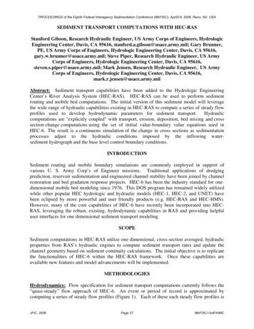
PROCEEDINGS of the Eighth Federal Interagency Sedimentation Conference (8thFISC), April2-6, 2006, Reno, NV, USAMODEL TESTING AND VERIFICATIONComparison to Myer-Peter and Muller Data: Several tests have been conducted to evaluatethese methodologies in HEC-RAS. First, HEC worked with Tony Thomas to simulate one of theoriginal Myer-Peter and Muller (MPM) experiments (1948) with HEC-RAS and HEC-6T. Sincethe MPM transport function was derived from these experiments, they can be simulated with anexpectation of reproducing the end result without the standard problems of transport functionuncertainty. In the MPM experiment, a constant flow was run through a flat bed flume with aconstant rate of gravel feed (grain size diameter 28.5mm) until it reached a stable, equilibriumslope of about 0.0081. This slope is plotted in Figure 3 with the equilibrium bed profilescomputed by HEC-6T and HEC-RAS. There was very good agreement between the physicaldata and both numerical models.Comparison of MPM Flume Data, and Simulations with HEC RAS and HEC 6TBed Elevation (ft)1.2Equilibrium Slope from MPM flume (d 28.5 mm) - 24hrs1.0Simulated Equilibrium Slope for HEC 6T (d 28.5 mm)- 24hrsSimulated Equilibrium Slope for HEC RAS (d 28.5 mm)- 24hrs0.80.60.40.20.0020406080100120140Flume Station (ft)Figure 3 Myer-Peter and Muller flume data with HEC-6 and HEC-RAS simulations.Comparison to HEC-6: There are several settings between HEC-6 and HEC-RAS that canproduce divergent results (e.g. fall velocity method, hydraulic radius vs. hydraulic depth, andfriction slope methods). In general, if these settings are harmonized, HEC-RAS does areasonably good job replicating HEC-6 (e.g. Figure 3).However, sometimes smallhydrodynamic differences can result in divergent sediment results. In the example depicted inFigure 4, Yang (1972) was applied to a trapezoidal channel with a single grain size material.Small differences in how HEC-6 and HEC-RAS compute water surface profiles resulted in aminor difference in calculated transport capacity ( 0.56%). However, since supply was onlyslightly larger than capacity, this small capacity discrepancy translated into a 6% difference intotal aggradation. Therefore the bed profiles diverge, despite very small calculated differences.It is of note that the computational differences implemented in RAS, though minor, areconsidered improvements by HEC and, therefore, the sediment responses to these are consideredto be improvements as well.JFIC, 2006Page 608thFISC 3rdFIHMC