WIXLIB

DIFFUSE OPTICAL LIGHT IN GALAXY CLUSTERS. II.has made its way into the ICL, either from ellipticals with lowmetallicity, spirals with younger stellar populations, or in situformation.While multiple mechanisms are likely to play a role in thecomplicated process of formation and evolution of clusters, important constraints can come from ICL measurement in clusterswith a wide range of properties. In addition to directly constraining galaxy evolution mechanisms, the ICL flux and color is a testable prediction of cosmological models. As such it can indirectlybe used to examine the accuracy of the physical inputs to thesemodels.This paper is structured in the following manner. In x 2 wediscuss the characteristics of the entire sample. Details of the observations and reduction are presented in xx 3 and 4, includingflat-fielding, sky background subtraction methods, object detection, and object removal and masking. In x 5 we list the results forboth cluster and ICL properties as well as accuracy limits. A discussion of the interesting correlations can be found in x 6, followedby a summary of the conclusions in x 7. Details of the individualclusters can be found in the Appendix. Throughout this paper weuse H0 ¼ 70 km s 1 Mpc 1, M ¼ 0:3, and ¼ 0:7.2. THE SAMPLEThe general properties of our sample of 10 galaxy clustershave been outlined in Paper I; for completeness we summarizethem briefly here and in Table 1. Our choice of the 10 clustersboth minimizes the observational hazards of the Galactic andecliptic plane and maximizes the amount of information in theliterature. All clusters were chosen to have published X-ray luminosities, which guarantees the presence of a cluster and providesan estimate of the cluster’s mass. The 10 chosen clusters are representative of a wide range in cluster characteristics, namely redshift (0:05 z 0:3), morphology (three with no clear centraldominant galaxy, and seven with a central dominant galaxy as determined from this survey [x 5.1.2] and not from Bautz-Morganmorphological classifications), spatial projected density (richnessclass 0Y3), and X-ray luminosity (1:9 ; 10 44 ergs s 1 LX 22 ; 10 44 ergs s 1). We discuss results from the literature andthis survey for each individual cluster in order of ascending redshift in the Appendix.3. OBSERVATIONSThe sample is divided into a ‘‘low’’ (0:05 z 0:1) and‘‘high’’ (0:15 z 0:3) redshift range, which we have observed with the 1 m Swope and 2.5 m du Pont telescopes, respectively. The du Pont observations were discussed in detail inPaper I. The Swope observations follow a similar observationalstrategy and data-reduction process, which we outline below. Observational parameters are listed in Table 2.We used the 2048 ; 3150 Site No. 3 CCD with a 3 e count 1gain and 7 e read noise on the Swope telescope. The pixel scaleis 0.43500 pixel 1 (15 m pixel 1), so that the full field of viewper exposure is 14:8 0 ; 22:8 0 . Data were taken in two filters, Gunnr (k0 ¼ 6550 8) and B (k0 ¼ 4300 8). These filters were selectedto provide some color constraint on the stellar populations in theICL by spanning the 4000 8 break at the relevant redshifts whileavoiding flat-fielding difficulties at longer wavelengths and prohibitive sky brightness at shorter wavelengths.Observing runs occurred on 1998 October 20Y26, 1999 September 2Y11, and 2000 September 19Y30. All observing runstook place within 8 days of new moon. A majority of the datawere taken under photometric conditions. Those images takenunder nonphotometric conditions were individually tied to the467photometric data (see discussion in x 4). Across all three runs,each cluster was observed for an average of 5 hr in each band. Inaddition to the cluster frames, night-sky flats were obtained innearby, off-cluster, ‘‘blank’’ regions of the sky with total exposure times roughly equal to one-third of the integration times oncluster targets. Night-sky flats were taken in all moon conditions.Typical B- and r-band sky levels during the run were 22.7 and21.0 mag arcsec 2, respectively.Cluster images were dithered by one-third of the field of viewbetween exposures. The large overlap from the dithering patterngives us ample area for linking background values from the neighboring cluster images. Observing the cluster in multiple positionson the chip reduces large-scale flat-fielding fluctuations on combination. Integration times were typically 900 s in r and 1200 sin B.4. REDUCTIONIn order to create mosaicked images of the clusters with auniform background level and accurate resolved-source fluxes,the images were bias and dark subtracted, flat-fielded, flux calibrated, background subtracted, extinction corrected, and registered before combining. Methods for this are discussed in detailin Paper I and summarized below.The bias level is roughly 270 counts, which changed by approximately 8% throughout the night. This, along with the largescale ramping effect in the first 500 columns of every row, wasremoved in the standard manner using IRAF tasks. The meandark level is 1.6 counts per 900 s, and there is some verticalstructure in the dark that amounts to 1.4 counts per 900 s over thewhole image. To remove this large-scale structure from the dataimages, a combined dark frame from the whole run was mediansmoothed over 9 ; 9 pixels (3:9 00 ), scaled by the exposure time,and subtracted from the program frames. Small-scale variationswere not present in the dark. Pixel-to-pixel sensitivity variationswere corrected in all cluster and night-sky flat images usingnightly, high signal-to-noise ratio (S/N), median-combined domeflats with 70,000Y90,000 total counts. After this step, a large-scaleillumination pattern remained across the chip. This was removedusing night-sky flats of ‘‘blank’’ regions of the sky, which, whencombined using masking and rejection, produced an image withno evident residual flux from sources but has the large-scale illumination pattern intact. The illumination pattern was stable amongimages taken during the same moon phase. Program images werecorrected only with night-sky flats taken in conditions of similarmoon.We find that the Site No. 3 CCD does have an approximately7% nonlinearity over the full range of counts, which we fit witha second-order polynomial and corrected for in all the data. Thesame functional fit was found for both the 1998 and 1999 data,and also applied to the 2000 data. The uncertainty in the linearitycorrection is incorporated in the total photometric uncertainty.Photometric calibration was performed in the usual mannerusing Landolt standards over a range of air masses. Extinctionwas monitored on stars in repeat cluster images throughout thenight. Photometric nights were analyzed together; solutions werefound in each filter for an extinction coefficient and common magnitude zero point with a r- and B-band rms of 0.04 and 0.03 magin 1998 October, 0.03 and 0.03 mag in 1999 September, and0.05 and 0.05 mag in 2000 September, respectively. These uncertainties are a small contribution to our final error budget (x 5.3).Those exposures taken in nonphotometric conditions were individually tied to the photometric data using roughly 10 starswell distributed around each frame to find the effective extinctionfor that frame. Among those nonphotometric images we find a

TABLE 1Cluster CharacteristicsCluster FluxCluster NameaA4059 .A3880a .A2734a .A2556a .A4010a .A3888.A3984a .A141a .AC 114.AC 118.M3 0.23b0.31l0.308b1:05 0:050:55 0:050:62 0:051:11 0:050:72 0:050:17 0:040:64 0:040:56 0:040:53 0:040:24 0:04RichnessClass1011122323Number ofGalaxies v( km s 1)76629910493189151185220288c845þ280 140e827þ120 79e628þ61 571247 249ce625þ127 95i1102þ137 107.i1388þ128 71n1947þ292 201rvirial( Mpc)d2.62.5f2.4d2.6f3.1f3.7d3.5f3.7f3.5m3.4mICL FluxRatioMass(1014 M )B(1011 L )r(1011 L )B(1011 L )r(1011 L )B(%)r(%)ICL Colord2:82þ0:37 0:34g8:3þ2:8 2:1d2:49þ0:89 0:63h4:2 1:33:8 1:13:4 1:03:3 0:993:5 1:07:2 2:24:4 1:35:4 1:62:3 0:705:4 1:612 3:58:6 2:612 3:613 3:812 3:730 9:020 6:032 9:518 5:344 1:31:2 :240:44 0:230:7 0:470:14 0:140:77 0:280:86 :250:62 0:210:34 0:110:38 0:080:67 0:173:4 1:71:4 0:462:8 0:470:76 0:663:2 0:704:4 2:12:2 1:03:5 0:882:2 0:47:0 0:9721 810 617 134 418 811 312 66 314 311 522 1214 619 66 521 813 510 610 411 214 51.892.632.542.482.541.971.492.722.152.7525 1g3:8þ1:6 1:2d25:5þ10:5 7:431 10jk18:9þ11:1 8:7þ8:2 i26:3 7:138 37iNote.—Sources for the virial radii and mass are discussed in xx A1 YA10 and generally come from X-ray data.aWe have obtained additional photometric and spectroscopic data for this cluster, which will be published in a forthcoming paper.bStruble & Rood (1999).cWu et al. (1999).dReiprich & Böhringer (2002).eGirardi et al. (1998a).fEbeling et al. (1996).gGirardi et al. (1998b).hReimers et al. (1996).iGirardi & Mezzetti (2001).jCypriano et al. (2004).kDahle et al. (2002).lAbell et al. (1989).mAllen (1998).nCouch & Sharples (1987).

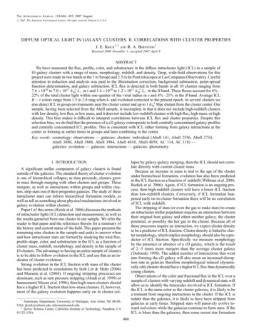
DIFFUSE OPTICAL LIGHT IN GALAXY CLUSTERS. II.469TABLE 2Observational ParametersExposure Time( hr)Native DetectionThreshold(mag arcsec 2 )Average Seeing(arcsec)Corrected DetectionThreshold(mag arcsec 2 )Background Accuracy(mag arcsec 2 )ClusterRedshiftrB or VrB or VField of View(h 170 Mpc)rB or VrB or VrB or VA4059.A3880.A2734.A2556.A4010.A3888.A3984.A141.AC 118.AC 1.41.30.91.01.01.01.81:2 ; 1:41:7 ; 2:21:7 ; 1:92:0 ; 2:42:3 ; 2:52:3 ; 2:22:3 ; 2:52:8 ; 2:72:7 ; 2:92:4 ; 029.829.929.8Notes.— The first five clusters in the table were imaged with the 1 m Swope telescope in the r and B bands. The last five clusters in the table were imaged with the2.5 m du Pont telescope in the r and V bands. Native detection threshold refers to the measured detection threshold of the cluster at its appropriate redshift. Correctedsurface brightness detection threshold refers to the actual detection threshold to which we mask at the redshift of each cluster. This detection threshold has been surfacebrightness dimmed and k-corrected to a redshift of 0, as discussed in x 4.2.2.standard deviation of 0.03 mag within each frame. Two furtherproblems with using nonphotometric data for low surface brightness (LSB) measurements are the scattering of light off of clouds,which causes a changing background illumination across the field,and, second, the smoothing out of the point-spread function (PSF).We find no spatial gradient over the individual frame to the limitdiscussed in x 5.3. The change in PSF is on small scales and willhave no effect on the ICL measurement (see x 4.2.1).Due to the temporal variations in the background, it is necessary to link the off-cluster backgrounds from adjacent frames tocreate one single background of zero counts for the entire clustermosaic before averaging together frames. To determine the background on each individual frame we measure average counts inapproximately 20 regions of 20 ; 20 pixels across the frame. Regions are chosen individually by hand to be a representative sample of all areas of the frame that are more distant than 0.8 h 170 Mpcfrom the center of the cluster. This is well beyond the radius atwhich ICL components have been identified in other clusters( Paper I; Feldmeier et al. 2002; Gonzalez et al. 2005; Zibettiet al. 2005). The average of these background regions for eachframe is subtracted from the data, bringing every frame to a zerobackground. The accuracy of the background subtraction is discussed in x 5.3.The remaining flux in the cluster images after backgroundsubtraction is corrected for atmospheric extinction by multiplying each individual image by 10 2:5, where is the air mass and is the fitted extinction in magnitudes from the photometric solution. This multiplicative correction is between 1.04 and 2.0 foran air mass range of 1.04Y1.9.The IRAF tasks geomap and geotran were used to find andapply x- and y-shifts and rotations between all images of a singlecluster. The geotran solution is accurate on average to 0.03 pixels(rms). Details of the final combined image after preprocessing,background subtraction, extinction correction, and registrationare included in Table 2.4.1. Object DetectionObject detection follows the same methods as Paper I. We useSExtractor to both find all objects in the combined frames and todetermine their shape parameters. The detection threshold in theV, B, and r images was defined such that objects have a minimumof six contiguous pixels, each of which are brighter than 1.5 above the background sky level. We choose these parametersas a compromise between detecting faint objects in high S/ N regions and rejecting noise fluctuations in low S/N regions. Thiscorresponds to minimum surface brightnesses that range from25.2 to 25.8 mag arcsec 2 in B, 25.9 to 26.9 mag arcsec 2 in V,and 24.7 to 26.4 mag arcsec 2 in r (see Table 2). This range insurface brightness is due to varying cumulative exposure timein the combined frames. Shape parameters are determined inSExtractor using only those pixels above the detection threshold.4.2. Object Removal and MaskingTo measure the ICL we remove all detected objects from theframe by either subtraction of an analytical profile or masking.Details of this process are described below.4.2.1. StarsScattered light in the telescope and atmosphere produce anextended PSF for all objects. To correct for this effect, we determine the extended PSF using the profiles of a collection of starsfrom supersaturated 4 mag stars to unsaturated 14 mag stars. Theradial profiles of these stars were fit together to form one PSFsuch that the extremely saturated star was used to create the profile at large radii and the unsaturated stars were used for the innerportion of the profile. This allows us to create an accurate PSF toa radius of 70 , shown in Figure 1.The inner region of the PSF is well fit by a Moffat function.The outer region is well fit by r 2:0 in the r band and r 1:6 in the Bband. In the r band there is a small additional halo of light atroughly 5000 Y10000 (200Y400 pixels) around stars imaged on theCCD. The newer, higher quality, antireflection-coated interference B-band filter does not show this halo, which implies thatthe halo is caused by reflections in the filter. To test the effect ofclouds on the shape of the PSF we create a second deep PSF fromstars in cluster fields taken under nonphotometric conditions.There is a slight shift of flux in the inner 1000 of the PSF profile,which will have no impact on our ICL measurement.For each individual, nonsaturated star, we subtract a scaledband-specific profile from the frame in addition to masking theinner 3000 of the profile (the region that follows a Moffat profile).For each individual saturated star, to be as cautious as possible

470KRICK & BERNSTEINFig. 1.— PSF of the 40 inch Swope telescope at Las Campanas Observatory.The y-axis shows surface brightness scaled to correspond to the total flux of a0 mag star. The profile within 500 was measured from unsaturated stars and canbe affected by seeing. The outer profile was measured from two stars with supersaturated cores imaged in two different bands. The profile with the bump in it at10000 is the r-band profile; that without the bump is the B-band PSF. The bumpin the profile at 10000 is due to a reflection off the CCD that then bounces off ofthe filter and back down onto the CCD. The outer surface brightness profile decreases as r 2 in the r band and r 1:6 in the B, shown by the dashed lines. Anr 3:9 profile is plotted to show the range in slopes.with the PSF wings, we have subtracted a stellar profile given theUSNO magnitude of that star and produced a large mask to coverthe inner regions and any bleeding. The mask size is chosen to betwice the radius at which the star goes below 30 mag arcsec 2,and therefore goes well beyond the surface brightness limit atwhich we measure the ICL. We can afford to be liberal with oursaturated star masking, since most clusters have very few saturated stars that are not near the center of the cluster where weneed the unmasked area to measure any possible ICL.In the specific case of A3880 there are two saturated stars(9 and 10 mag, r band) within 20 of the core region of the cluster.If we used the same method of conservatively masking (twice theradius of the 30 mag arcsec 2 aperture), the entire central regionof the image where we expect to find ICL would be lost. Wetherefore consider a less extreme method of removing the stellarprofile by iteratively matching the saturated stars’ profiles withthe known PSF shape. We measure the saturated star profiles onan image that has had every object except for those two saturatedstars masked, as described in x 4.2.2. We can then scale our measured PSF to the star’s profile, at radii where there is expected tobe no contamination from the ICL, and the star’s flux is not saturated. Since the two stars are within 10 of each other, the scaledprofiles of the stars are iteratively subtracted from the maskedcluster image until the process converges on solutions for the scaling of each star. We still use a mask for the inner region ( 7500 )where saturation and seeing effect the profile shape.4.2.2. GalaxiesWe want to remove all the flux in our images associated withgalaxies. Although some galaxies might follow de Vaucouleurs,Sérsic, or exponential profiles, those galaxies that are near thecenters of clusters cannot be fit with these or other models either,Vol. 134because of the overcrowding in the center or because their profiles really are different due to their location in a dense environment. A variety of strategies for modeling galaxies within thecenters of clusters were explored in Paper I and were found to beinadequate for these purposes. Since we cannot fit and subtractthe galaxies to remove their light, we instead mask all galaxies inour cluster images.By masking, we remove from our ICL measurements all pixels above a surface brightness limit that are centered on a galaxyas detected by SExtractor. For Paper I, we chose to mask insideof 2Y2.3 times the radius at which the galaxy light dropped below 26.4 mag arcsec 2 in r, akin to 2Y2.3 times a Holmbergradius (Holmberg 1958). Holmberg radii are typically used todenote the outermost radii of the stellar populations in galaxies.Galaxy profiles will also have the characteristic underlying shapeof the PSF, including the extended halo. However, for a 20 maggalaxy, the PSF is below 30 mag arcsec 2 by a radius of 1000 .Each of the clusters has a different native surface brightness detection threshold based on the illumination correction andbackground subtraction, and they are all at different redshifts.However, we want to mask galaxies at all redshifts to the samephysical surface brightness to allow for a meaningful comparison between clusters at different redshifts. To do this wemake a correction for (1 þ z) 4 surface brightness dimming and ak-correction for each cluster when calculating mask sizes. Themask sizes change by an average of 10% and at most 22% fromwhat they would have been given the native detection threshold.Both the native and corrected surface brightness detection thresholds are listed in Table 2. To test the effect of mask size on the ICLprofile and total flux, we also create masks that are 30% larger and30% smaller in area than the calculated mask size. The flux withinthe masked areas for these galaxies is on average 25% more thanthe flux identified by SExtractor as the corrected isophotal magnitude for each object.5. RESULTSHere we discuss our methods for measuring both cluster andICL properties, as well as a discussion of each individual clusterin our sample.5.1. Cluster PropertiesCluster redshift, mass, and velocity dispersion are taken fromthe literature, where available, as listed in Table 1. Additionalproperties that can be identified in our data, particularly thosethat may correlate with ICL properties (cluster membership, flux,dynamical state, and global density), are discussed below andalso summarized in Table 1.5.1.1. Cluster Membership and FluxCluster membership and galaxy flux are both determined using a color-magnitude diagram (CMD) of either B r versus r(clusters with z 0:1) or V r versus r (clusters with z 0:1).We create CMDs for all clusters using corrected isophotal magnitudes as determined by SExtractor. Membership is then assigned based on a galaxy’s position in the diagram. If a givengalaxy is within 1 of the red cluster sequence ( RCS) determined with a biweight fit, then it is considered a member (fits areshown in Fig. 2). All others are considered to be nonmemberforeground or background galaxies. This method selects the redelliptical galaxies as members. The benefits of this method arethat membership can easily be calculated with two-band photometry. The drawbacks are that it both does not include someof the bluer true members and does include some of the redder

No. 2, 2007DIFFUSE OPTICAL LIGHT IN GALAXY CLUSTERS. II.471Fig. 2.— CMDs for all 10 clusters in increasing redshift order from left to right and top to bottom: A4059, A3880, A2734, A2556, A4010, A3888, A3984, A141,AC 114, and AC 118. All galaxies detected in our image are denoted with an asterisk. Those galaxies that have membership information in the literature are overplottedwith triangles (members) or squares (nonmembers) (membership references are given in xx A1 YA10). Solid lines indicate a biweight fit to the red sequence with 1 uncertainties.nonmembers. An alternative method of determining cluster fluxwithout spectroscopy by integrating under a background-subtractedluminosity function is discussed in detail in x 5.3 of Paper I. Dueto the large uncertainties involved in both methods ( 30%), thechoice of procedure will not greatly affect the conclusions.To determine the total flux in galaxies, we sum the flux of allmember galaxies within the same cluster radius. The image sizeof our low-redshift clusters restricts that radius to one-quarter ofthe virial radius of the cluster where virial radii are taken from theliterature or calculated from X-ray temperatures as described inxx A1YA10. From tests with those clusters where we do havesome spectroscopic membership information from the literature(see xx A3 and A6), we expect the uncertainty in flux from usingthe CMD for membership to be 30%.Fits to the CMDs produce the mean color of the red ellipticals,the slope of the color-magnitude relation (CMR) for each cluster,

472KRICK & BERNSTEINVol. 134Fig. 2 — Continuedand the width of that distribution. Among our 10 clusters, thecolor of the red sequence is correlated with redshift, whereas theslopes of the relations are roughly the same across redshift, consistent with López-Cruz et al. (2004). The widths of the CMRsvary from 0.1 to 0.4 mag. This is expected if these clusters aremade up of multiple c

Rudick et al. 2006). Again, if ICL formation is an ongoing pro-cess, then high-redshift clusters will have a lower ICL fraction than low-redshift clusters. Conversely, if ICL formation hap-pened early on in cluster formation there will be no correlation of ICL with redshift. The stripping of stars (or even the gas to make stars) to create