WIXLIB

Repayment and default regions: period 13.0Bond price schedulelow K1high K10.62.50.5Default at low K1Always repay2.01.5Qe1low K1high K10.70.40.31.00.2Always default0.50.10.00.00.00 0.25 0.50 0.75 1.00 1.25 1.50 1.75 2.00b10.00 0.25 0.50 0.75 1.00 1.25 1.50 1.75 2.00bFigure 2: Repayment region and bond price scheduleIn period 0, households solve the maximization problem (1) taking the loan schedule (3) asgiven. We write the fraction of borrowers that choose to default in period 0 as d0 . A key questionfor us is how d0 varies with penalties K0 and the level of GDP y0 . We study these questions insections 2.2 and 4.2, respectively.For their part, savers simply smooth consumption across the two periods. They face no incomeuncertainty, have log utility, and discount the future at rate βS . They collect labor income, whichis y0 in period 0 and 1 in period 1, as well as the profits made by the intermediary. Their problem,taking into account the value Π of intermediary shares, is therefore: max log c0S βS log c1Ss.t. c0S c1S1 y0 ΠRRGiven that the intermediary makes no profits on any loan between date 0 and date 1, the value ofthe intermediary starting from date 0 is just the value of the legacy debts that are repaid:Π (1 d0 ) b0Equilibrium.Household consumption is the only source of demand for goods. Denoting byc0B(e0 ) the consumption policy of a borrower with income shock e0 , aggregate consumption inperiod 0 is defined as:Z11c0 c0B (e0 ) dF (e0 ) c0S22similarly, denoting by c1B (e1 , b1 ) the consumption policy of a borrower with income shock e1 anddebt b0 in period 1, and by b1 (e0 ) the debt policy in period 0, aggregate consumption in period 1is defined as:1c1 2Z Z1c1B (e1 , b1 (e0 )) dF (e1 ) dF (e0 ) c1S26

In a small open economy, R, y0 and y1 1 are all given. The economy starts period 0 and endsperiod 1 with no net claim to the rest of the world. Any excess of absorption c0 over productiony0 in period 0 is resolved by net imports in period 0, and net exports in period 1.In a demand determined economy, R and y1 1 are also given, but y0 adjusts to clear the goodsmarket in period 0,4 that is:c0 y0By Walras’s law, the goods market then also clears in period 1.Policy-maker tools and objectives.We assume that the policymaker can choose K0 and K1 . Thispolicymaker may be interested in raising the level of consumption c0 , the level of equilibriumshort-run output y0 , or in maximizing societal welfare, placing a certain weight λ on savers:W Z Z u c0B (e0 ) βu c1B (e0 , e1 ) dF (e0 ) dF (e1 ) λ u c0S βS u c1Swhere u (c) log c.2.2Ex-post debt reliefWe first study the macroeconomic and welfare implications of changing the default laws in period0 in a completely unexpected way, as captured in our model by changing K0 .Period 0 default decision.A household entering period 0 with income shock e0 chooses theaction that maximizes the value in (1). We write c0r (e0 ) for the policy function in case of repayment,and c0d (e0 ) for the policy in case of default. We further define the Consumption Effect of Defaultat e0 , or CED, as:CED (e0 ) c0d (e0 ) c0r (e0 )b0 Q (b1 (e0 )) b0b0(4)The CED is the additional consumption that a given household enjoys over a certain period if hedefaults rather than repays, normalized by his level of debt. It is also the share of that household’sdebt that he repays rather than roll over. Since higher income households tend to save more(borrow less), the CED is increasing in income e0 . Moreover, the CED is tightly connected toincentives to repay rather than default. Indeed, the envelope theorem and log utility togetherimply that, at all levels of income, 0( V r ) 0 ( e0 ) V d ( e0 )c0d (e0 ) c0r (e0 )c0d (e0 ) CEDe ()0u0 (c0r (e0 ))b0c0d (e0 )(5)4 We can microfound this assumption by assuming that the central bank is at the zero lower bound and and achievesno inflation.7

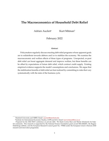
Values of repaying and defaulting0.0Always0.5 defaultDefault at low K0Consumption Effect of Default (CED)0.30Always repay0.251.00.201.50.152.00.102.5Always0.05 defaultVrV d, low K0V d, high K03.03.50.20.40.6e00.81.00.001.2Default at low K00.20.40.6Always repaye00.81.01.2Figure 3: Values of repaying and defaulting and the Consumption Effect of DefaultIn this paper, we focus on the case where the CED is positive at the lowest level of income. Bymonotonicity, it is then positive at all levels of income. Equation (5) then implies that the differencebetween V r and V d grows with e0 , so that there is a single intersection e0 such that V r (e0 ) V d (e0 ). Figure 3 illustrates this situation in a calibrated example. On the left, the black line V rhas steeper slope than the orange line V d , so the two value functions intersect at a unique pointe0 . On the right, we see that the CED is positive throughout. Since the default region is [0, e0 ],5 thedefault rate is:d 0 F ( e0 )Consider what happens to this default rate as the policymaker lowers K0 . This raises the valueof defaulting (to the blue line in Figure 3), without affecting the value of repaying. Hence, thethreshold e0 moves to the right, and the default rate d0 increases. This argument shows that thepartial derivative of d0 with respect to K0 is negative, d0 K0 0.The open economy. We are ready to consider the general equilibrium implications of debt relief.We first consider debt relief in the small open economy (soe).Proposition 1. In the small open economy, a marginal change in K0 affects aggregate consumption according to: c0 K0 soe b d00 ACED MPC S · ·2 K0(6)where ACED CED (e0 ) 0 is the consumption effect of default at the indifference threshold, andMPC S 11 β Sis the marginal propensity to consume of savers.5 While this situation can be shown to be the only one in some special cases (e.g. Arellano 2008) and is fairly generic in quantitative models, in the general case, the default region is a segment e0 , e0 (e.g. Chatterjee et al. 2007, Mitman2016), with households repaying at incomes below e0 . In that case, the CED is negative in the lower repayment region,as poorer borrowers prefer to borrow to sustain their consumption above the level that they can achieve in default.8

The intuition for Proposition 1 is as follows. Consider debt relief, with the policymaker lowering penalties by dK0 0. Most borrowers do not change their decisions in terms of eitherdefaulting or spending, but a mass dd0 d0 K0 dK0 0 of marginal borrowers with income e0switches over from repaying to defaulting on their debt. The effect on spending from this additional consumption is ACED · b20 · dd0 . At the same time, financial intermediaries make lossesb0S b02 · dd0 , which they pass on to savers. In turn, savers cut consumption by MPC · 2 · dd0 . Thenet effect on aggregate spending then depends on the balance between the ACED and the MPC S ,scaled by the level of debt and the effect on the default rate.This argument shows that default constitutes redistribution between savers and borrowers,and that the ACED (the causal effect of defaulting on spending) is the correct way of evaluatingthe effect of that redistribution on aggregate borrower spending. While here we study a simplecase with a single marginal type, in general there are many marginal types. What matters then isa certain average CED across these types, hence the term ACED.While we saw that theory naturally predicts that the ACED is positive, the MPC S is also positive. However, in a permanent-income calibration, MPC S would be quite low (in an infiniteβhorizon model interpretation, βS 1 β , and MPC S 1 β), while data from defaulters suggeststhat the ACED may be quite high (see section 3.2). Hence, Proposition 1 suggests that the effect ofdebt relief on aggregate spending is likely to be positive.We next turn to the study of welfare. We prove the following:Proposition 2. In the small open economy, a marginal change in K0 affects aggregate welfare according to: W K0 soe d 0 d0 λu c0S b0 K00The intuition is simple. The first term, d0 , is the marginal social benefit of lower default penalties. Debt relief dK0 0 directly raises by one util the utility of the fraction d0 of borrowers who aredefaulting. Some borrowers also switch to defaulting rather than repaying, but these are marginalborrowers who were already indifferent between their two options, so this does not affect socialwelfare. The second term is the marginal social cost of these lower penalties: they raise the default d0rate by dd0 KdK0 0, so impose losses on all savers of b0 · dd0 , and these are valued at λu0 c0S0 by the planner. If the planner places low enough weight on savers (λu0 c0S is low enough), thendebt relief can raise welfare.Proposition 2 shows that the benefits of the lower penalties from debt relief are perceived byall the defaulters in the same way. This contrasts with transfers, which would raise social welfare according to the average marginal borrower utility u0 c0B . This suggests that debt relief operatesin a different space than some other redistributive instruments, and may be helpful in conjunctionwith these instruments to raise social welfare.Demand determined economy.We now briefly consider the case of a demand-determined econ-omy, studied in much more detail in Auclert and Mitman (2022). This is relevant since aggregate9

demand externalities are often invoked in discussions of debt relief.Proposition 3. In the demand-determined economy, a marginal change in K0 affects equilibrium outputaccording to: where M 1 c1 y0 y0 K0 dd M· c0 K0 soe(7)is the economy’s multiplier, i.e. the sensitivity of output to a change in demand.0In the small open economy, the increase in spending from debt relief dK0 0 leads to anincrease in the economy’s imports. By contrast, in a demand-determined economy, it leads tomore spending on domestic goods, raising domestic incomes and therefore spending accordingto the economy’s aggregate MPC c0 y0 .The equilibrium effect on output is the initial soe effect 2 c0 c0multiplied by the standard Keynesian multiplier M 1 y · · · . In equilibrium, this y00amplifies the aggregate demand effect of debt relief.Proposition 4. In the demand-determined economy, a marginal change in K0 affects welfare according to: W K0 dd W K0 soe τ·M· c0 K0 soe(8)where τ is the sensitivity of welfare to an increase in aggregate demand.When the economy is demand-determined, an increase in aggregate demand may be beneficialfor welfare (τ 0). In that case, the welfare benefits of debt relief captured in proposition 2 areamplified by the presence of an aggregate demand demand externality, as captured by the secondterm in (8) (see e.g. Farhi and Werning 2016, Korinek and Simsek 2016).Taking stock.Unexpected debt relief can boost aggregate spending provided that the spendingeffect on defaulters (the ACED) is larger than that on those who pay for it (the MPC S ). It can alsoraise social welfare if the policymaker perceives the weight on those who pay for the debt reliefto be low enough (low λ), and may even be better at achieving this objective than direct transfersto defaulters. Finally, there may be additional benefits if the economy is depressed, since then theincreased aggregate spending has a multiplier effect on output, and social welfare may be furtherhelped by the resultant increase in output if there is an aggregate demand externality.While we have made the case that the ACED is likely larger than the MPC S , we note that ourmodel assumes a frictionless banking system. In practice, financial frictions can cause losses inthe banking system to propagate to declines in aggregate output (e.g. Gertler and Kiyotaki 2010).In the language of our model, this would raise the MPC S , possibly above the ACED. However,this effect can be avoided by taxing savers, or borrowing from future taxpayers, to recapitalize thebanking system.10

2.3Expected debt reliefWe now study the effect of an announcement at date 0 of debt relief at date 1. Recall that, asFigure 2 showed, a decline in penalties for period 1 (K1 ) shifts in credit supply and lowers the Q 0). This has important implications foramount that borrowers receive in the first period ( K1the aggregate demand effects of expected debt relief.We first observe that, contrary to the unexpected change in K0 , which affected previouslywritten contracts, a change in K1 has no effect on saver spending, since banks pass through thehigher expected defaults to borrowers in the form of higher spreads, to the point that they do notmake losses. On the other hand, borrower spending is affected because of the direct shift in creditsupply and the indirect response of borrowers to it.Proposition 5. In the small open economy, a marginal change in K1 affects aggregate consumption according to: c0 K1 soe 11 Q E e0(b1 ) 2 K12{z} direct effectE e0 b1 Q(b1 ) b1 K1{z} 0(9)indirect effect through change in borrowingWe saw in section 2.1 that the direct effect of a decline in K1 , holding borrowing decisionsfixed, is always negative. In principle, borrowers could offset the effects of this shift on their consumption by borrowing more. The behavioral response involves an income effect, a substitutioneffect, and a precautionary saving effect. It is possible to show that these effects are never enoughto undo the direct effect of the credit supply shift, so that announced future debt relief dK1 0always leads to a decline in aggregate spending dc0soe 0.Turning to welfare, we have the following result:Proposition 6. In the small open economy, a marginal change in K1 affects welfare according to: W K1 soe βEe0 [d1 ] Ee0 u0 c0B,r Q K1(10)Here, savers are on their Euler equation, so their welfare is not affected by the change in thetiming of cash flows induced by the change in K1 . The aggregate effect on welfare therefore onlyreflects how borrower welfare is affected. The envelope theorem implies that there are only twoeffects from announced future debt relief (dK1 0). First, a direct benefit to all future defaulters,similar to Proposition 2. Second, a marginal cost from the increased difficulty in borrowing todayas credit supply is reduced. See Dávila (2020) for a closely connected result.Propositions 5 and 6 capture all the economics of expected relief. In the demand-determined debtsoesoesoe c0 c0dWby Kin (9) and dKeconomy, propositions 3 and 4 apply directly, but replacing K011 soedWby dK1in (10). Hence, if expected debt relief leads to a contraction in credit supply and there-fore spending, the effect on output will be aggravated because of the multiplier M, and the effecton welfare will be lower because of the aggregate demand externality τ.11

3Supporting empirical evidenceIn this section, we discuss recent micro and macro evidence that supports the assumptions andthe aggregate predictions of our model. For a more detailed discussion of the micro evidence onhousehold debt relief in its various forms, see Indarte (2021) in this volume.3.1Legal framework in the United StatesIt is useful here to briefly summarize the details of the consumer bankruptcy system in the U.S. toclarify the types of variation that past empirical studies have exploited to make inference on theeffect of debt relief on various economic outcomes. Bankruptcy in the U.S. is the legal procedurefor discharging personal debts. A unique feature of the U.S. bankruptcy code is that it is a so-called“fresh start” system, whereby at the end of the bankruptcy procedure all debts are discharged andcreditors have no claims on future income.6 Furthermore, debtors are not required to surrenderall of their property and assets when filing. Each state can determine the type and amount ofproperty that is exempt from seizure in bankruptcy. Households have the option of filing undertwo different parts of the code: Chapter 7 or 13. Chapter 7 is “liquidation” whereby all non-exemptproperty is seized and then all unsecured debts are canceled. Chapter 13 entails a three to five yearrepayment plan where households can keep all of their assets, but are obliged to contribute all oftheir discretionary income to debt payments, after which any remaining debt is canceled. Thevast majority of households file under Chapter 7 (which is analogous to default in our theoreticalframework), so the remainder of this section will focus on aspects of Chapter 7 bankruptcy.7When a household files for bankruptcy, it has to declare all of its assets and unsecured liabilitiesto the court. In theory, any non-exempt assets are seized and liquidated, and the proceeds aretransferred to creditors. In practice, more than 95% of bankruptcy cases result in no assets beingseized by the court. The primary asset that households can keep in bankruptcy is their primaryresidence. The so-called homestead exemption varies significantly across states, from a low of 5,000 in Kentucky, to an unlimited amount in states like Florida and Texas. The relative generosityof exemptions has been remarkably stable over time, and thus the variation in exemptions hasbeen frequently used in cross-sectional analyses for inference.After filing, households are precluded from filing again for six years. The bankruptcy “flag”remains on the credit report for 10 years after the filing date. This implies that household access tounsecured credit is limited (Han and Li 2011) and remains so persistently until the flag is removedfrom the credit report (Musto 2004, Herkenhoff 2019). These institutional features motivate ourmodeling choice of exclusion from unsecured borrowing after a default in the model period 0.6 Bycontrast, in most European countries bankruptcy serves more as debt restructuring, whereby individuals areliable for the rest of their lives until the debt is repaid in full.7 Throughout the rest of the paper we will slightly abuse language and refer to Chapter 7 bankruptcy as bankruptcyor default. A separate strand of the literature has focused on “informal default” where househol

0 captures pure ex-post debt relief, since lenders have no time to change the terms of debt contracts. By contrast, the effect of changing K 1 on date-0 outcomes captures the ex-ante effect of an announcement of future debt relief. In this section, we assume that the policymaker can independently manipulate K 0 and K 1. We come back to this .