Transcription
Image and Vision Computing 25 (2007) 262–273www.elsevier.com/locate/imavisA sensitivity analysis method and its application in physics-basednonrigid motion modeling*Yong Zhang a,*, Dmitry B. Goldgof b,1, Sudeep Sarkar b, Leonid V. Tsap cbaDepartment of Computer Science and Information Systems, Youngstown State University, Youngstown, OH 44555, USADepartment of Computer Science and Engineering, University of South Florida, 4202 East Fowler Avenue, Tampa, FL 33620, USAcAdvanced Communications and Signal Processing Group, Electronics Engineering Department,University of California Lawrence Livermore National Laboratory, Livermore, CA 94551, USAReceived 19 October 2004; received in revised form 4 June 2005; accepted 4 August 2005AbstractParameters used in physical models for nonrigid and articulated motion analysis are often not known with high precision. It has been recognizedthat commonly used assumptions about the parameters may have adverse effect on modeling quality. In this paper, we present an efficientsensitivity analysis method to assess the impact of those assumptions by examining the model’s spatial response to parameter perturbation.Numerical experiments with a synthetic model and skin tissues show that: (1) normalized sensitivity distribution can help determine the relativeimportance of different parameters; (2) dimensional sensitivity is useful in the assessment of a particular parameter assumption; and (3) models aremore sensitive at the locations of property discontinuity (heterogeneity). The formulation of the proposed sensitivity analysis method is generaland can be applied to assessment of other types of assumptions, such as those related to nonlinearity and anisotropy.q 2006 Elsevier B.V. All rights reserved.Keywords: Sensitivity analysis; Physical modeling; Nonrigid motion; Elastic parameters1. IntroductionDuring the past two decades, physics-based modeling hasemerged as one of the most important techniques for nonrigidand articulated motion analysis [18]. Its popularity is evidencedby the increasing number of publications each year as well asthe diversity of the fields in which the papers appeared. Forexample, physical model has found applications in: nonrigidand articulated motion tracking [21,22,15,34], realistic facialanimation [19,17], surgery simulation and operation planning[6,3,7], elastic medical image registration [4,36,14], dynamiccloud simulation using satellite images [33], as well as shaperepresentation and recognition [25,24], to name a few. More*Part of this work was performed under the auspices of the US Departmentof Energy by University of California Lawrence Livermore NationalLaboratory under contract number W-7405-Eng-48. UCRL-JRNL-207977.* Corresponding author. Tel.: C1 330 941 1786; fax: C1 330 941 2284.E-mail addresses: yzhang@cis.ysu.edu (Y. Zhang), goldgof@cse.usf.edu(D.B. Goldgof), sarkar@cse.usf.edu (S. Sarkar), tsap@llnl.gov (L.V. Tsap).1Tel.: C1 974 4055/974 2113; fax: C1 813 974 4055/2113.0262-8856/ - see front matter q 2006 Elsevier B.V. All rights sive survey and in-depth discussions on physicsbased nonrigid motion analysis can be found in [1,20].In comparison to geometrical and mass-spring models,physical models that are based on continuum mechanics havehigh computational complexity. As a result, various assumptions are often made to simplify the model and its parameters.For example, a commonly used assumption is that the materialproperties of an object are isotropic and homogeneous.However, results from large amount of biomechanical tests[12] indicate that the mechanical behavior of many biologicalmaterials, especially soft tissues, cannot be accuratelydescribed by such a simplified model. Certain types of muscles(such as skeletal muscle) are characterized by stronganisotropic behaviors. More importantly, the property heterogeneity of several orders of magnitude is also common inhuman organs [9]. Recently, measuring elastic property ofabnormalities caused by the pathological processes has beenutilized for early cancer detection [11,10].Recognizing the inadequacy of simplified physical models,researchers have started to investigate to what degree the variousassumptions, especially those about the material properties andthe boundary conditions, may affect the model’s performanceby means of sensitivity analysis. For example, Alterovitz et al.[2] studied the influence of both the physician-controlled
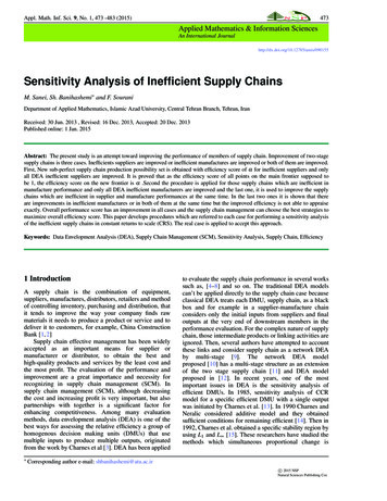
Y. Zhang et al. / Image and Vision Computing 25 (2007) 262–273263parameters and the intrinsic material parameters on the accuracyof needle insertion simulation. In the study of model-basedbreast cancer diagnosis, Tanner et al. [28] compared the resultsof biomechanical models with different settings of boundarycondition and material properties. However, those studies weredone on the case-by-case basis using ad hoc comparisonmethods, and therefore the conclusions cannot be readilygeneralized to other domains. Moreover, the experiments wereperformed based on the assumption that the model hashomogeneous material properties, which implies that thesolution of a Dirichlet type problem could be independent ofthe internal property variation, and hence the subsequentsensitivity analysis results may not be valid. Another limitationof their methods is that the sensitivity data is incapable ofproviding a complete picture of the model’s spatial response tothe parameter variation on each individual point of the model.In this paper, we propose a local gradient based computationmethod that can be used to conduct a systematic andcomprehensive sensitivity analysis of any motion model.Specifically, physics-based nonrigid motion modeling willbenefit from such a sensitivity analysis in the followingaspects:problem [37,12], and then discuss the derivation of the adjointstate equation and related computational issues.1. The proposed method allows us to compare the relativeimportance of different parameters using the normalizedsensitivity data and quantify the impact of variousassumptions on model’s performance using the dimensionalsensitivity data;2. The algorithm is designed based on the adjoint statemethod, which significantly reduces the computational costand is suited for handling large scale finite element models;3. The sensitivity contour map enables us to identify thevulnerable areas of a model that are most affected by a poorassumption, so that further improvement can be made;4. The parameter value can be obtained by either the directmeasurement [12] or the indirect inference [23]. But thoseacquisition procedures are time-consuming and expensive.It would be economic to first conduct a sensitivity analysisto identify the primary parameters and then to concentrateour effort on the acquisition of those parameters.where u denotes the displacement vector, r is the mass density,t denotes the time, s is the stress tensor, T denotes the transposeoperator, B is the body force, P is the divergence operatorwith respect to a tensor, 3 is the strain tensor, tr denotes trace, Iis the identity matrix, l and m are the Lamé constants, P is the gÞ are thegradient operator defined with respect to a vector, ðu;Dirichlet and Neumann data on the boundary (G1,G2) thatdefine the modeling domain U, and n is the outward unitnormal on the boundary (see Fig. 1).Eqs. (1)–(3) are also known in continuum mechanics as themotion equation, the constitutive equation and the straindisplacement equation, respectively. Material propertiescommonly used in the engineering literature such as theYoung’s modulus (E) and the Poisson’s ratio (n) are related tothe Lamé constants by:2.1. Primary problemThe deformation of an elastic body can be described by thefollowing partial differential equations and the boundaryconditions (primary problem)rv2 uZ V sT C B;vt2in U Z G1 C G2 ;s Z lðtr3ÞI C 2m3 Z lðV uÞI C mVu C mðVuÞT ;(2)13 Z ½Vu C ðVuÞT ;2(3) on G1 ;u Z u;(4)vu on G2 ;Z g;vn(5)mZE;2ð1 C nÞ2. Sensitivity analysisSensitivity analysis is closely related to optimizationproblems often encountered in the traditional model calibrationtasks, such as optimal shape design, boundary conditionspecification, discretization strategy investigation, as well asmaterial property assignment [16]. In this study, we focus onassessing the impact of two elastic parameters (the Young’smodulus and the Poisson’s ratio) on model’s performance,based on the computed sensitivity information. Without loss ofgenerality, we will discuss the deformation of a linear elasticbody and its response to parameter perturbation. However, themethodology developed here can be readily applied tononlinear systems. We will give a brief review of the primary(1)Fig. 1. Illustration of the primary problem.(6)
264lZY. Zhang et al. / Image and Vision Computing 25 (2007) 262–273nE:ð1 C nÞð1K2nÞ(7)A variational method can be used to derive the finiteelement formulation of the above partial differential equationsso that a numerical solution of the forward model can beobtained. For example, using the Galerkin method [37], theprimary problem in the static equilibrium can be discretizedinto a linear finite element systemKu Z b;(8)where K is the stiffness matrix, u denotes the nodal solution,and b is the load vector.For each finite element, an interpolation matrix (Ri) (thebasis function) is used to relate the displacements in the localelement coordinate (di) and the global coordinate (u), whichensures that the requirement of strain compatibility is satisfied:di Z Ri u:(9)After the discretization, the corresponding constitutive Eq.(2) and the strain-displacement Eq. (3) in the discrete matrixform aresi Z Ki 3i ;(10)3i Z Di u;(11)where Ki is the coefficient of stiffness matrix and Di is a matrixderived from the spatial differentiation of Ri and thecombination of row items. Note that Ki is comprised of thematerial properties (E,n) that will be studied in the sensitivityanalysis.With the above notations, the stiffness matrix and the loadvector in (8) that assemble all the finite elements becomeKZM ðXiZ1bZRTi q1i dV CVM ðXiZ1SRTi q2i dS CLXq3j ;NameUrBP Iu G1UEKRq2Pts3Pl,mg G2NnBdiq3DDisplacementMass densityBody forceDivergenceIdentity matrixDirichlet dataDirichlet boundaryModeling domainYoung’s modulusStiffness matrixBasis functionSurface tractionGeneric parameterTimeCauchy stress tensorSmall strain tensorGradientLamé constantsNeumann dataNeumann boundaryoutward unit normalPoisson’s ratioLoad vectorLocal coordinatePoint loadDerived matrix of Rmodulus and the Poisson’s ratio: pZ{pj}Z{Ej , ni},jZ1,2,.M.All the variables and parameters discussed in this section arelisted in Table 1.2.2. Performance measure and dimensional sensitivityThe simplest sensitivity analysis method that can be done innonrigid motion modeling is based on a Taylor seriesdescribing the relationship between the state variable (u) andthe parameter (p)(13)uðp C DpÞ Z uðpÞ CjZ1where M is the total number of elements, V denotes the size ofelement, q1i is the body force within an element, q2i is thesurface traction term, q3j is the point load, and L is the numberof point loads exerted on the body.Since we are interested in the sensitivity assessment of amechanical system governed by (8) to the parameter variations,we rewrite (8) in terms of the parameter vectorKðpÞu Z bðpÞ;Variable(12)VM ðXiZ1DTi Ki Di dV;Table 1Variables and parameters in primary problem(14)where p denotes the generic parameter to be investigated,which could be the material properties, the stress or straindistributions, the loading conditions (either the Dirichlet typeor the Neumann type), object’s geometrical configuration, andeven the meshing scheme itself. Here, we concentrate on thesensitivity analysis of two spatial parameters, the Young’s!MXvu1Dpj Cvpj2jZ1M XMXv2 uDp Dp C .vpj vpl j ljZ1 lZ1(15)where the first-order derivatives (vu/vpj) are the coefficients ofthe Jacobian matrix: JZ[vui/vpj], (iZ1,2,.N; jZ1,2,.M)with N and M as the total number of nodes and the total numberof elements in a model, respectively.The Jacobian matrix provides a local description of theresponse of the state variable to the parameter change and isadequate for analyzing a simple system such as the mass-springmodel. However, for most practical engineering problems,more sophisticated sensitivity analysis method is needed tohelp us understand how a given model depends on certainparameters, so that the most significant ones can be identifiedand improved. To this end, a performance function (objective
Y. Zhang et al. / Image and Vision Computing 25 (2007) 262–273function) has to be defined:ðHðu;pÞ ZCombining (20) and (22), we have:f ðu; pÞdU:(16)dHðu;pÞZdpð U vf ðu; pÞ vf ðu; pÞ duCdU;vpvu dp(17)or in the discrete form:S Z ½S1 ;S2 ;.Sj ;.SM ;dHðu;pÞ vHðu;pÞ vHðu;pÞ duSj ZZC:dpjvpjvudpj(18)(19)Without causing any confusion, from now on, we willrepresent (18) and (19) with a single expression:SZdHðu;pÞ vHðu;pÞ vHðu;pÞ duZC:dpvpvudp(20)2.3. Adjoint state methodThe dimensional sensitivity can be computed using the finitedifference approximation, the direct differentiation or theadjoint state method [5]. We choose the adjoint state methodbecause it is more efficient for large scale problems. For a finiteelement model of modest size that are commonly encounteredin physics-based nonrigid motion simulation, the number ofelements could easily reach a couple of thousands. Therefore,the direct computation of sensitivity distribution would be toocostly.The adjoint state method is based on the principle ofvariational calculus [13], and can be derived from thegoverning partial differential equations in the continuousspace (1)–(5), or from the linear system in the discrete space(14). We will discuss the adjoint state approach following thesecond route.We first differentiate (14) with respect to the parameter pvKðpÞdu vbðpÞu C KðpÞ Z;vpdpvp(21)We then multiply (21) by an arbitrary vector 4 (adjoint statevariable)fTdHðu;pÞ vHðu;pÞ vHðu;pÞ duduZCKfT KðpÞdpvpvudpdpUThe function defined in (16) is only a generic integral form.The exact formula of f(u,p) is often task-dependent, and the useof Euclidean norm is common.Given a performance function H(u,p), we can define thedimensional sensitivity (S) as its total derivative with respect tothe parameter vectorSZ265vKðpÞduvbðpÞu C fT KðpÞ Z fT:vpdpvp(22)KfTvKðpÞvbðpÞu C fTvpvp(23)Since f is arbitrary, we chose a f such that the followingequation is satisfied (the second and third terms in the right sideof (23))vHðu;pÞ duduKfT KðpÞ Z 0:vudpdp(24) is equivalent to T T duduvHðu; pÞ TTK ðpÞf Z;dpdpvuwhich leads to the adjoint state equation vHðu;pÞ TKðpÞf Zvu(24)(25)(26)In the above derivation, we took advantage of the fact that thestiffness matrix is symmetric. Also note that the adjointproblem (26) is in the same form as the primary problem (14),except for the load term, (vH(u,p)/vu)T, which is also known asthe pseudo-load.Substituting (24) back into (23), we obtain: dHðu;pÞ vHðu;pÞvKðpÞT vbðpÞZCfKu :(27)SZdpvpvpvpAs a result, we only need to solve the primary problem (14)and the adjoint problem (26) once, in order to obtain the statesolution (u) and the adjoint state solution (f), and then use (27)to compute the dimensional sensitivity. The adjoint stateformulation can also be derived using the Lagrange multipliermethod by treating (14) as the state equation, (16) as aconstraint function and f as the Lagrange multiplier [8].2.4. Derivative computationThe partial derivative terms in (27) are needed in order tocalculate the dimensional sensitivity. If the performancefunction is defined in an explicit form, we can directlycompute the second term in (27) as:ðvHðu;pÞvf ðu;pÞZdU:(28)vpvpUIn most applications, f(u,p) is defined as a function of thestate variable only, f(u), and therefore its partial derivative withrespect to the parameter becomes zero.With a finite element formulation, the partial derivatives ofthe stiffness matrix (K) and the load vector (b) with respect tothe parameter (p) can be expressed as:M ðvKðpÞ XvKi ðpÞZDi dV;DTi(29)vpvpViZ1
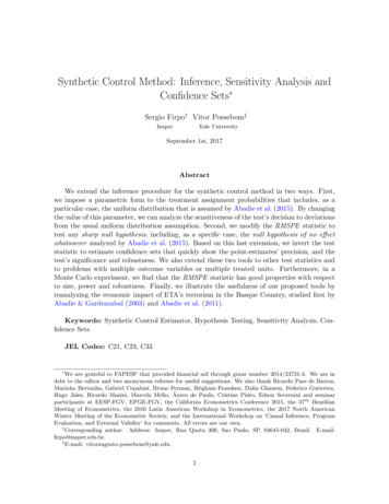
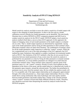
266Y. Zhang et al. / Image and Vision Computing 25 (2007) 262–273ðVRTiM ðXvq1i ðpÞvq2i ðpÞdV CdSRTivpvpSiZ1MXvq3j ðpÞCiZ1vp10 cm(30)Since we are interested in the sensitivity values with respect tothe material properties only (pZ{E,n}), the derivativecomputations involved in (29) and (30) will only cause aslight increase of the computational cost.8 cmMvbðpÞ XZvpiZ1Fixed3 (cm)Fixed3 (cm)Fixed3 (cm)Fixed3 (cm)3 (cm)Fixed2.5. Normalized sensitivityE 50 kPav 0.460Dimensional sensitivity as defined in (20) is suitable forstudying the dependence of a model on a single parameter (notethat the vector pZ[p1,p2,.,pM] of a finite element model isviewed as a single parameter here). Because each physicalparameter usually has its own unit, a comparison amongdifferent parameters such as the Young’s modulus and thePoisson’s ratio using the dimensional sensitivity is verydifficult and potentially could be misleading. In order toremove the dimensional effect, we define a normalizedsensitivity (Sn) as:pdHðu;pÞHðu;pÞdp pvHðu;pÞ vHðu;pÞ duCZHðu;pÞvpvudpE 500 kPav 0.495Fig. 2. Synthetic model configuration.pression loads are exerted along the right side boundary(displacementZ3 cm). The nodes on the top and bottomboundaries are set free.With the true parameters and boundary conditions as are generated byspecified above, the observation data ðuÞrunning a forward simulation. The data vector is defined on all ½u 1 ;u 2 ;.u N T Þ. It should be noted that, in realnodes ðuZapplications, the state variable may be measured only on partsof the object.Sn Z3.2. Performance measure(31)The normalized sensitivity measures the percentage changeof the performance function to the percentage change ofparameters. Therefore, it allows us to evaluate and rank theimportance of different parameters in terms of their impact onthe model on a common basis. Note that the normalizedsensitivity does not require any changes of the computationalprocedure (adjoint state method) developed for the dimensionalsensitivity. If the statistical information about the measurementdata is available, a normalized sensitivity function weighted bythe measurement confidence coefficient can also be considered.3. Experiments with a synthetic model3.1. Model configurationThe model used in this experiment represents a 2D elasticobject that has a size of 10!8 (cm2). The object is discretizedinto a finite element mesh with 357 nodes and 320 elements(Fig. 2). The elements are of quadrilateral thin shell type. Allelements are assigned with isotropic properties (EZ50 kPa,nZ0.460), except for the 32 elements in the middle of themodeling domain that have higher values (EZ500 kPa, nZ0.495), creating the property heterogeneity. This heterogeneously distributed properties are regarded as the trueparameters: ptZ{Et,nt}. The Dirichlet boundary conditionsare specified as follows: all nodes on the left side boundary ofthe model are fixed (displacementZ0 cm), while the com-We first define a performance function in the form ofdiscrete Euclidean norm:ðHðuÞ ZUf ðuÞdU Z jjf ðuÞjj2 ZNXw2i ½ui ðpa ÞKu i 2(32)iZ1where wi is a weight coefficient assigned to the ith node, padenotes the assumed parameters, u(pa) is the solution that isobtained using the assumed parameters and u represents theobservation data that is generated with the true parameters.In all of the experiments, we used the unit weight coefficient:wiZ1.This performance function consists of the state variableonly. So the marginal sensitivity (the second term in (27))becomes zero. In situations where the parameter measurementsare available, they can also be incorporated into theperformance function (H(u,p)). If stress or strain analysis isof interest, they can also be included to construct a Neumanntype performance function.Since homogeneity is a commonly used assumption, wetest a model that has the assumed homogeneous properties:paZ{EaZ50 kPa, naZ0.460}. The deformed models with thetrue heterogeneous properties (ptZ{Et,nt}) and the assumedhomogeneous properties (paZ{Ea,na}) are shown in Fig. 3.The discrepancy between the two deformed shapes is clearlyvisible. Next, we will demonstrate that (1) the normalizedsensitivity can be used to identify the parameter that is mostresponsible for the discrepancy; (2) the dimensional sensitivityis helpful for determining how good an assumption is.
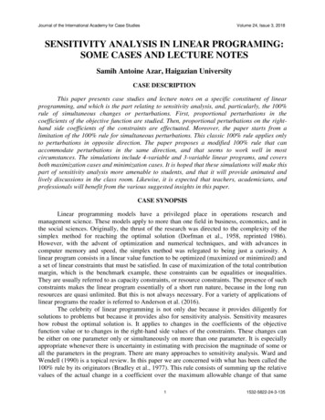
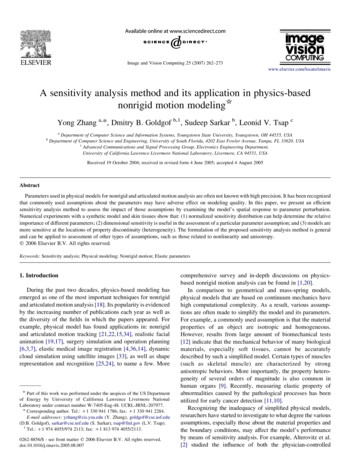
Y. Zhang et al. / Image and Vision Computing 25 (2007) 262–273267Fig. 3. Deformed models using (a) the true heterogeneous properties and (b) the assumed homogeneous properties.3.3. Normalized sensitivity distributionlocation of parameter abnormalities to which effort should bededicated to correct the original homogeneous assumption.The normalized sensitivities with respect to the Young’smodulus and the Poisson’s ratio are presented in Fig. 4. Thesensitivity distribution is plotted element by element as acontour map (SnZ[Sn1,Sn2,.SnM]T). The sensitivity coefficientin an element (Snj) represents the percentage change of theperformance function due to a 1% change of the parametervalue in that element. The difference between the two maps interms of the magnitude of sensitivity coefficient suggests thatthe model is more sensitive to the Young’s modulus than to thePoisson’s ratio. In other words, with this particular modelconfiguration, Young’s modulus has a significant impact on themodeling accuracy, while the effect of the Poisson’s ratio issecondary. It should be noted that a model of different settingsof Young’s modulus and Poisson’s ratio could show differentnormalized sensitivity distribution. However, it is always validto determine the relative significance of two parameters basedon their normalized sensitivity distributions, because thevariation in the magnitude of parameters has been compensatedwith the normalization process.Further inspection of Fig. 4(a) reveals that the model is mostsensitive at the property discontinuities. The geometry of thehigh sensitivity area matches the shape of property heterogeneity. So, the sensitivity map is also informative about the(a)3.4. Dimensional sensitivity distributionIt should be pointed out that certain formulations of theperformance function may result in a sensitivity value ofinfinity. For example, with a performance function as definedin (32), the examination of (31) suggests that, as the assumedparameters approach the true parameters (pa/pt), thenormalized sensitivity goes to infinity (Sn/N). Although itrarely occurs in real applications that our first assumption is asgood as the true parameters, it is still wise to interpret thenormalized sensitivity with cautions.In the context of nonrigid motion modeling, we recommenda two-step sensitivity analysis procedure: (1) the normalizedsensitivity can be used to quantify the relative importance ofparameters in terms of their impact on the model’s behavior;(2) once a parameter is considered as significant, thedimensional sensitivity can be used to assess the assumptionsabout the parameter. Without much loss of rigor, the closer theassumed parameters (pa) are to the true parameters (pt), thesmaller the dimensional sensitivity is. This statement is basedon the assumption that good correspondence data is available.Inaccurate correspondence data could complicate the sensitivity distribution and its interpretations, because a large(b)0.210.010.430.590.680.800.850.850.06 0.040.020.020.800.680.590.430.010.21Sn of theYoung's modulusSn of the Poisson's ratioFig. 4. Normalized sensitivity contour maps.0.04 0.06
268Y. Zhang et al. / Image and Vision Computing 25 (2007) .1e-104.9e-101.6e-122.6e-10S with Ehetero 440 kPaS with Ehetero 70 kPaFig. 5. Dimensional sensitivity contour maps.dimensional sensitivity value could be caused by either a badparameter assumption or the errors in correspondence data.Therefore, more work is needed to deal with the corruptedcorrespondence data.We experimented with two assumptions about the Young’smodulus inside the area of heterogeneity (the 32 elements inthe center of the model): E1Z70 and E2Z440 kPa. TheYoung’s modulus in the background elements and thePoisson’s ratio are the same as the true values. The dimensionalsensitivity contours using those two assumptions are shown inFig. 5 (unitZ[m/pa]). The smaller magnitude of the secondmap indicates that the assumption (E2Z440 kPa) is muchcloser to the true value (EtZ500 kPa) and is a betterassumption than the first one (E1Z70 kPa). In the study ofparameter estimation, the inverse algorithms also utilize thesensitivity information, although the regularization is moreimportant in solving the ill-posed inverse problems [36].3.5. Relative error distributionThe distribution of relative modeling error can alsocharacterize the complex relationship between a model’sbehavior and its parameters. The relative modeling error isdefined as follows:err Z juðpa ÞKuj: juj(33)(a)To determine the contribution to the relative modeling errorby an individual parameter, we carried out two experiments,one with the true heterogeneous Young’s modulus and theassumed homogeneous Poisson’s ratio, and one with theassumed homogeneous Young’s modulus and the trueheterogeneous Poisson’s ratio. The results are shown inFig. 6. The errors caused by an incorrect homogeneousassumption of the Young’s modulus is around 10–40%,while the errors due to a bad assumption of the Poisson’sratio is less than 0.08%, which confirms the conclusion drawnfrom the sensitivity analysis that the Young’s modulus is moresignificant than the Poisson’s ratio under the configuration ofthis synthetic model.4. Experiments with burn scarThe experiment with synthetic model has implications tomany practical modeling problems, because the propertyvalues used in the experiment are based on the publisheddata. For example, in needle insertion simulation, a Young’smodulus in the range of 40–160 kPa was used for prostatetissue [2]. In breast modeling, the variation of E amongdifferent tissues can be up to an order of magnitude, 10–88 kPafor the skin tissue and 1–184 kPa for glandular tissue [3,28].The Poisson’s ratio used in soft tissue modeling is often in therange of 0.465–0.495. Therefore, the modeling scenario ofsynthetic model is very realistic and the sensitivity 40.00030.03err with Ea and νterr with Et and νaFig. 6. Relative error distributions. Et: true Young’s modulus, Ea: assumed Young’s modulus, nt: true Poisson’s ratio, na: assumed Poisson’s ratio.
Y. Zhang et al. / Image and Vision Computing 25 (2007) 262–273269Fig. 7. Deformation of burn scar.A patient’s arm with a burn scar was used in the experiment.Using an ink stamp, a rectangle grid was created on the arm’ssurface. Two images were then taken before and after thepatient’s arm was stretched (see Fig. 7). A finite element modelwith quadrilateral thin shell element was then constructed thatmatches the rectangle grid (see [29] for detailed descriptions ofthe modeling procedure). A Dirichlet condition was specifiedaround the boundary using the measured displacement data andthe internal nodes were set free.of E and n is not as large as those observed in the experimentswith synthetic model.It can be seen that the region of high normalized sensitivityvalues matched well with the overall shape of scar (in both theYoung’s modulus map and the Poisson’s ratio map). Thissimilarity between the scar boundary and the sensitivitycontours indicates that the model is very sensitive to theproperty change between scar and normal skin. It has beenobserved that the Young’s modulus of the burn scars could be2–10 times higher than that of the normal skin (5–100 kPa)[29]. Based on the normalized sensitivity map of the Poisson’sratio in Fig. 8(b), it seems reasonable to expect that the sametype of heterogeneity of Poisson’s ratio exists between the scarand the normal skins, although the magnitude of theheterogeneity still remains unclear.4.2. Normalized sensitivity4.3. Dimensional sensitivityThe finite element model covers both the scar (in themiddle) and the surrounding normal skins. A homogeneousproperty distribution throughout the model was assumed forboth the Young’s modulus and the Poisson’s ratio (EZ60 kPa,nZ0.495). The normalized sensitivity contours computed withthe above setting are shown in Fig. 8. Again, the larger valuesin Fig. 8(a) indicate that the scar model is more sensitive to thechange of the Young’s modulus than to that of the Poisson’sratio, although the difference between the sensitivity valuesA homogeneous elasticity assumption is certainly notadequate for scar assessment study. We use the next exampleto demonstrate how to find a better assumption based on thedimensional sensitivity information. We gradually increasedthe Young’s modulus value of scar (eight elements in themiddle of the model) from the initial 60 kPa until no furtherimprovement can be observed in terms of the model’sdimensional sensitivity distribution. To quantify the evaluationprocess, we used an average dimensional sensitivity value:demonstrated with the synthetic model can be readily extendedto real objects. In the next experiment, we will apply thesensitivity method to burn scar.4.1. Model 40.020.160.030.060.02Sn of theYoung's modulusSn of the Poisson's ratioFig. 8. Normalized sensitivity maps of scar.0.04
270Y. Zhang et al. / Image and Vision Computing 25 (2007) 2.0e-118.1e-113.2e-11S with Escar 60 kPa7.2e-12 5.8e-12S with Escar 450 kPaFig. 9. Dimensional sensitivity maps of scar.Save ZM1 XS:M jZ1 j(34)As discussed in the previous section, the smaller Save is, thecloser the corresponding assumption is to the true distribution.The fina
A sensitivity analysis method and its application in physics-based nonrigid motion modeling* Yong Zhang a,*, Dmitry B. Goldgof b,1, Sudeep Sarkar b, Leonid V. Tsap c a Department of Computer Science and Information Systems, Youngstown State University, Youngstown, OH 44555, USA b Department of Computer Science and Engineering, University of South Florida, 4202 East Fowler Avenue, Tampa, FL .